Example: Virtual circuit calculations

---

This example notebook will demonstrate how to construct virtual circuits (VCs) for a MAST-U-like tokamak equilibrium.

What are Virtual Circuits and why are they useful?

VCs can be used to identify which (active) poloidal field (PF) coils have the most significant impact on a set of specified plasma shape parameters (which we will refer to henceforth as targets). The targets are equilibrium-related quantities such as the inner or outer midplane radii \(R_{in}\) or \(R_{out}\) (more will be listed later on).

More formally, the virtual circuit (VC) matrix \(V\) for a given equilibrium (and chosen set of shape targets and PF coils) is defined as

\[ V = (S^T S)^{-1} S^T, \]

where \(S\) is the shape (Jacobian) matrix:

\[ S_{i,j} = \frac{\partial T_i}{\partial I_j}. \]

Here, \(T_i\) is the \(i\) th target and \(I_j\) is the current in the \(j\) th PF coil. We note that \(V\) is simply the Moore-Penrose pseudo-inverse of \(S\). In FreeGSNKE, \(S\) will be calculated using finite difference (see below).

How can these VCs be used?

Once we know the VC matrix \(V\) for a given equilibrium (and its associated target values \(\vec{T}\)), we can specify a perturbation in the targets \(\vec{\Delta T}\) and calculate the change in coil currents required to acheive the new targets. The shifts in coil currents can be found via:

\[ \vec{\Delta I} = V \vec{\Delta T}. \]

Using \(\vec{\Delta I}\) we can perturb the coil currents in our equilibrium, re-solve the static forward Grad-Shafranov (GS) problem, and observe how the targets (call them \(\vec{T}_{new}\)) have changed in the new equilibrium vs. the old targets \(\vec{T}\).

---

Generate a starting equilibrums

Firstly, we need an equilbirium to test the VCs on.

import numpy as np
import matplotlib.pyplot as plt

# build machine
from freegsnke import build_machine
tokamak = build_machine.tokamak(
    active_coils_path=f"../machine_configs/MAST-U/MAST-U_like_active_coils.pickle",
    passive_coils_path=f"../machine_configs/MAST-U/MAST-U_like_passive_coils.pickle",
    limiter_path=f"../machine_configs/MAST-U/MAST-U_like_limiter.pickle",
    wall_path=f"../machine_configs/MAST-U/MAST-U_like_wall.pickle",
    magnetic_probe_path=f"../machine_configs/MAST-U/MAST-U_like_magnetic_probes.pickle",
)

# initialise the equilibrium
from freegsnke import equilibrium_update
eq = equilibrium_update.Equilibrium(
    tokamak=tokamak,
    Rmin=0.1, Rmax=2.0,   # Radial range
    Zmin=-2.2, Zmax=2.2,  # Vertical range
    nx=65,                # Number of grid points in the radial direction (needs to be of the form (2**n + 1) with n being an integer)
    ny=129,               # Number of grid points in the vertical direction (needs to be of the form (2**n + 1) with n being an integer)
    # psi=plasma_psi
)  

# initialise the profiles
from freegsnke.jtor_update import ConstrainPaxisIp
profiles = ConstrainPaxisIp(
    eq=eq,        # equilibrium object
    paxis=8e3,    # profile object
    Ip=6e5,       # plasma current
    fvac=0.5,     # fvac = rB_{tor}
    alpha_m=1.8,  # profile function parameter
    alpha_n=1.2   # profile function parameter
)

# load the nonlinear solver
from freegsnke import GSstaticsolver
GSStaticSolver = GSstaticsolver.NKGSsolver(eq)    

# set the coil currents
import pickle
with open('data/simple_diverted_currents_PaxisIp.pk', 'rb') as f:
    current_values = pickle.load(f)
for key in current_values.keys():
    eq.tokamak.set_coil_current(key, current_values[key])

# carry out the foward solve to find the equilibrium
GSStaticSolver.solve(eq=eq, 
                     profiles=profiles, 
                     constrain=None, 
                     target_relative_tolerance=1e-4)

# updates the plasma_psi (for later on)
eq._updatePlasmaPsi(eq.plasma_psi)

# plot the resulting equilbria 
fig1, ax1 = plt.subplots(1, 1, figsize=(4, 8), dpi=80)
ax1.grid(True, which='both')
eq.plot(axis=ax1, show=False)
eq.tokamak.plot(axis=ax1, show=False)
ax1.set_xlim(0.1, 2.15)
ax1.set_ylim(-2.25, 2.25)
plt.tight_layout()

Active coils --> built from pickle file.
Passive structures --> built from pickle file.
Limiter --> built from pickle file.
Wall --> built from pickle file.

Magnetic probes --> built from pickle file.

Resistance (R) and inductance (M) matrices --> built using actives (and passives if present).
Tokamak built.

Forward static solve SUCCESS. Tolerance 5.98e-05 (vs. requested 1.00e-04) reached in 19/100 iterations.

Initialise the VC class

We initialise the VC class and tell it to use the static solver we already initialised above. This will be used to repeatedly (and rapidly) to solve the static GS problem when calculating the finite differences for the shape matrix.

from freegsnke import virtual_circuits

VCs = virtual_circuits.VirtualCircuitHandling()
VCs.define_solver(GSStaticSolver)

Define shape targets

Next we need to define the shape targets (i.e. our quantities of interest) that we wish to monitor.

The way we do this is exactly the same as was seen in Example05b with the “plasma_descriptors” function. The user just needs to define a function that takes in the eq as a (single) input and returns an array of the shape targets (sometimes called parameters) of interest. See the function defined in the next cell.

# define the descriptors function (it should return an array of values and take in an eq object)
def plasma_descriptors(eq):

    # inboard/outboard midplane radii
    RinRout = eq.innerOuterSeparatrix()

    # inboard midplane radius
    Rout = eq.innerOuterSeparatrix()[0]

    # find lower X-point
    # define a "box" in which to search for the lower X-point
    XPT_BOX = [[0.33, -0.88], [0.95, -1.38]]

    # mask those points
    xpt_mask = (
        (eq.xpt[:, 0] >= XPT_BOX[0][0])
        & (eq.xpt[:, 0] <= XPT_BOX[1][0])
        & (eq.xpt[:, 1] <= XPT_BOX[0][1])
        & (eq.xpt[:, 1] >= XPT_BOX[1][1])
    )
    xpts = eq.xpt[xpt_mask, 0:2].squeeze()
    if xpts.ndim > 1 and xpts.shape[0] > 1:
        opt = eq.opt[0, 0:2]
        dists = np.linalg.norm(xpts - opt, axis=1)
        idx = np.argmin(dists)  # index of closest point
        Rx, Zx = xpts[idx, :]
    else:
        Rx, Zx = xpts

    return np.array([RinRout[0], RinRout[1], Rx, Zx])

Assign these shape targets some decriptive names (and ensure the names are in the correct order!). You can then call the function to test it works correctly.

target_names = ["Rin", "Rout", "Rx", "Zx"]
target_values = plasma_descriptors(eq)

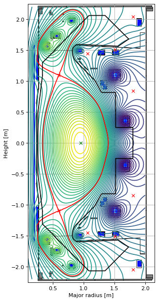
Let us visualise the targets on our equilibrium.

# plot the resulting equilbria 
fig1, ax1 = plt.subplots(1, 1, figsize=(4, 8), dpi=80)
ax1.grid(True, which='both')
ax1.contour(eq.R, eq.Z, eq.psi(), levels=[eq.psi_bndry], colors='r')
eq.tokamak.plot(axis=ax1, show=False)
ax1.plot(eq.tokamak.wall.R, eq.tokamak.wall.Z, color='k', linewidth=1.2, linestyle="-")

ax1.scatter(target_values[0], 0.0, s=100, color='green', marker='x', zorder=20, label=target_names[0])
ax1.scatter(target_values[1], 0.0, s=100, color='blue', marker='x', zorder=20, label=target_names[1])
ax1.scatter(target_values[2], target_values[3], s=100, color='m', marker='*', zorder=20, label=f"({target_names[2]},{target_names[3]})")

ax1.set_xlim(0.1, 2.15)
ax1.set_ylim(-2.25, 2.25)
ax1.legend(loc="upper right")
plt.tight_layout()

Calculating the VCs

Now we’ve defined the targets we’re interested in, we can begin calculating the shape and virtual circuit matrices. The following is a brief outline of how they’re calculated:

1. Initialise and solve the base equilibrium

Before computing derivatives, the static forward GS solver is run with some initial coil currents. Following this we store the:

• equilibrium state eq and plasma profiles profiles.

• plasma current vector \(I_y\) (which defines the amount of plasma current at each computational grid point, restricted to the limiter region to save computational resources).

• target values \(\vec{T} = [T_1,\ldots,T_{N_T}]\) are evaluated.

This establishes a reference state before we perturb the coil currents - we have already carried out these steps above (the \(I_y\) vector is stored within profiles).

2. Find the appropriate coil current perturbations

Next, we need to identify the appropriate coil current perturbations \(\vec{\delta I}\) to use in the finite differences. To do this, we aim to scale the starting guess starting_dI (denoted \(\vec{\delta I}^{start}\)) according to the target tolerance on the plasma current vector (target_dIy = \(\delta I_y^{target}\)). While the user can choose starting_dI, the default is given by

\[ \vec{\delta I}^{start} := | \vec{I} | \times \delta I_y^{target}. \]

For each coil current \(j \in \{1,\ldots,N_c \}\), this starting guess is scaled as follows:

1. Perturb coil current \(j\):

\[ I_j^{new} := I_j + \delta I_j^{start}.\]

2. Solve the equilibrium with the updated \(j\) th coil current (others are left unchanged) and store the plasma current vector \(\vec{I}_y^{new}\).

3. The starting guess for the \(j\) th coil current perturbation is then scaled by the relative norm of the plasma current change (and the predefined target tolerance target_dIy):

\[ \delta I_j^{final} = \delta I_j^{start} \times \left( \delta I_y^{target} \frac{\| \vec{I}_y^{start} \|}{\| \vec{I}_y^{new} - \vec{I}_y^{start} \|} \right).\]

If this relative norm is larger than \(\delta I_y^{target}\), then the starting guess \(\delta I_j^{start}\) needs to be made smaller (and vice versa).

After this, we have our scaled perturbations \(\vec{\delta I}^{final}\) ready to use in the finite differences.

3. Find the finite differences (i.e. the shape matrix)

For each coil current \(j \in \{1,\ldots,N_c \}\):

1. Perturb coil current \(j\):

\[ I_j^{new} := I_j + \delta I_j^{final}.\]

2. Solve the equilibrium with the updated \(j\) th coil current (others are left unchanged) and store the plasma current vector \(\vec{I}_y^{new}\).

3. Using the new target values \(\vec{T}^{new}\) from the equilibrium, calculate the \(j\) th column of the shape matrix:

\[ S_{:,j} = \frac{\vec{T}^{new} - \vec{T}}{\delta I_j^{final}}. \]

This gives the sensitivity of each of the targets \(T_i\) with respect to a change in the \(j\) th coil current.

Note that we can also obtain the Jacobian matrix of the plasma current vector (using \(\vec{I}_y^{new}\)) with respect to the coil currents: \(\frac{\partial \vec{I}_y}{\partial \vec{I}}\).

4. Find the virtual circuit matrix

Once the full shape matrix \(S \in \Reals^{N_T \times N_c} \) is known, the virtual circuit matrix is computed as:

\[ V = (S^T S)^{-1} S^T \in \Reals^{N_c \times N_T}.\]

This matrix provides a mapping from requested shifts in the targets to the shifts in the coil currents required.

# next we need to define which coils we wish to calculate the shape (finite difference) derivatives (and therefore VCs) for
print("All active coils :", eq.tokamak.coils_list[0:12])

# here we'll look at a subset of the coils and the targets
coils = ['PX', 'D1', 'D2', 'D3', 'Dp', 'D5', 'D6', 'D7', 'P4', 'P5']
print("Coils to calculate VCs for :", coils)

All active coils : ['Solenoid', 'PX', 'D1', 'D2', 'D3', 'Dp', 'D5', 'D6', 'D7', 'P4', 'P5', 'P6']
Coils to calculate VCs for : ['PX', 'D1', 'D2', 'D3', 'Dp', 'D5', 'D6', 'D7', 'P4', 'P5']

# calculate the shape and VC matrices using the in-built method
VCs.calculate_VC(
    eq=eq,
    profiles=profiles,
    coils=coils,
    target_names=target_names,
    target_calculator=plasma_descriptors,
    starting_dI=None,    
    min_starting_dI=50,
    verbose=True,
    name="VC_for_lower_targets", # name for the VC
    )

--- Stage one ---
Re-sizing each initial coil current shift so that it produces a 0.1% change in plasma current density from the input equilibrium.

Forward static solve SUCCESS. Tolerance 1.13e-08 (vs. requested 1.00e-07) reached in 5/100 iterations.
Coil PX (original current shift = 50.0 [A] --> scaled current shift 27.05 [A]).

Forward static solve SUCCESS. Tolerance 9.21e-09 (vs. requested 1.00e-07) reached in 4/100 iterations.
Coil D1 (original current shift = 50.0 [A] --> scaled current shift 19.79 [A]).
Forward static solve SUCCESS. Tolerance 1.69e-08 (vs. requested 1.00e-07) reached in 3/100 iterations.
Coil D2 (original current shift = 50.0 [A] --> scaled current shift 20.14 [A]).

Forward static solve SUCCESS. Tolerance 7.47e-09 (vs. requested 1.00e-07) reached in 4/100 iterations.
Coil D3 (original current shift = 50.0 [A] --> scaled current shift 15.24 [A]).

Forward static solve SUCCESS. Tolerance 5.95e-08 (vs. requested 1.00e-07) reached in 4/100 iterations.
Coil Dp (original current shift = 50.0 [A] --> scaled current shift 6.41 [A]).

Forward static solve SUCCESS. Tolerance 1.40e-08 (vs. requested 1.00e-07) reached in 5/100 iterations.
Coil D5 (original current shift = 50.0 [A] --> scaled current shift 4.27 [A]).

Forward static solve SUCCESS. Tolerance 6.93e-09 (vs. requested 1.00e-07) reached in 4/100 iterations.
Coil D6 (original current shift = 50.0 [A] --> scaled current shift 4.4 [A]).

Forward static solve SUCCESS. Tolerance 3.75e-08 (vs. requested 1.00e-07) reached in 4/100 iterations.
Coil D7 (original current shift = 50.0 [A] --> scaled current shift 3.8 [A]).

Forward static solve SUCCESS. Tolerance 6.43e-08 (vs. requested 1.00e-07) reached in 4/100 iterations.
Coil P4 (original current shift = 50.0 [A] --> scaled current shift 2.6 [A]).

Forward static solve SUCCESS. Tolerance 2.50e-08 (vs. requested 1.00e-07) reached in 5/100 iterations.
Coil P5 (original current shift = 50.0 [A] --> scaled current shift 1.32 [A]).
--- Stage two ---
Building the shape matrix (Jacobian) of the shape parameter changes wrt scaled current shifts for each coil:
Coil PX

Forward static solve SUCCESS. Tolerance 4.35e-08 (vs. requested 1.00e-07) reached in 6/100 iterations.
Coil D1

Forward static solve SUCCESS. Tolerance 4.37e-08 (vs. requested 1.00e-07) reached in 3/100 iterations.
Coil D2
Forward static solve SUCCESS. Tolerance 8.80e-09 (vs. requested 1.00e-07) reached in 4/100 iterations.
Coil D3

Forward static solve SUCCESS. Tolerance 1.18e-08 (vs. requested 1.00e-07) reached in 3/100 iterations.
Coil Dp

Forward static solve SUCCESS. Tolerance 4.04e-08 (vs. requested 1.00e-07) reached in 3/100 iterations.
Coil D5
Forward static solve SUCCESS. Tolerance 2.57e-08 (vs. requested 1.00e-07) reached in 3/100 iterations.
Coil D6

Forward static solve SUCCESS. Tolerance 2.72e-08 (vs. requested 1.00e-07) reached in 3/100 iterations.
Coil D7

Forward static solve SUCCESS. Tolerance 1.26e-08 (vs. requested 1.00e-07) reached in 3/100 iterations.
Coil P4
Forward static solve SUCCESS. Tolerance 7.45e-08 (vs. requested 1.00e-07) reached in 2/100 iterations.
Coil P5

Forward static solve SUCCESS. Tolerance 3.84e-08 (vs. requested 1.00e-07) reached in 4/100 iterations.
--- Stage three ---
Inverting the shape matrix to get the virtual circuit matrix.
VC object stored under name: 'VC_for_lower_targets'.

# these are the finite difference derivatives of the targets wrt the coil currents
shape_matrix = 1.0*VCs.VC_for_lower_targets.shape_matrix
print(f"Dimension of the shape matrix is {shape_matrix.shape} [no. of targets x no. of coils]. Has units [m/A]")

# these are the VCs corresponding to the above shape matrix
VCs_matrix = 1.0*VCs.VC_for_lower_targets.VCs_matrix
print(f"Dimension of the virtual circuit matrix is {VCs_matrix.shape} [no. of coils x no. of targets]. Has units [A/m].")

Dimension of the shape matrix is (4, 10) [no. of targets x no. of coils]. Has units [m/A]
Dimension of the virtual circuit matrix is (10, 4) [no. of coils x no. of targets]. Has units [A/m].

How do we make use of the VCs?

Now that we have the VCs, we can use them to idenitfy the coil current shifts required to change the targets by a certain amount.

For example, we will ask for shifts in a few shape targets and observe what happens to the equilibrium once we apply the new currents from the VCs.

# let's remind ourselves of the targets
print(target_names)

['Rin', 'Rout', 'Rx', 'Zx']

# let's set the requested shifts (units are metres) for the full set of targets
requested_target_shifts = [0.05, -0.05, 0.0, 0.0]

We specify a perturbation in the targets \(\vec{\Delta T}\) (the shifts above) and calculate the change in coil currents required to achieve this by calculating:

\[ \vec{\Delta I} = V \vec{\Delta T}. \]

Using \(\vec{\Delta I}\) we then perturb the coil currents in our original equilibrium, re-solve the static forward Grad-Shafranov (GS) problem, and return. This is all done in the following cell.

# we apply the VCs to the desired shifts, using the VC_object we just created
eq_new, profiles_new, new_target_values, old_target_values = VCs.apply_VC(
    eq=eq,
    profiles=profiles,
    VC_object=VCs.VC_for_lower_targets,
    requested_target_shifts=requested_target_shifts,
    verbose=True,
)

Currents shifts from VCs:
['PX', 'D1', 'D2', 'D3', 'Dp', 'D5', 'D6', 'D7', 'P4', 'P5'] = [ 3204.78715603    84.30254267  -303.61395742  -231.96924695
 -1079.72993551   233.27811588   299.69387068   553.76719085
  1551.27404662 -1033.40653128].

Targets shifts from VCs:
['Rin', 'Rout', 'Rx', 'Zx'] = [ 0.05278377 -0.04646511  0.00104334 -0.00363978].

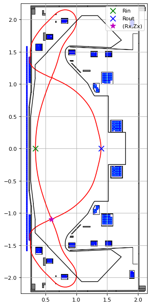
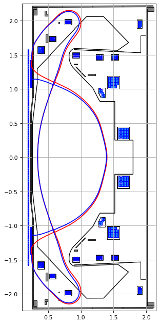
# plot the resulting equilbria 
fig1, ax1 = plt.subplots(1, 1, figsize=(4, 8), dpi=80)
ax1.grid(True, which='both')
ax1.plot(eq.tokamak.wall.R, eq.tokamak.wall.Z, color='k', linewidth=1.2, linestyle="-")
eq.tokamak.plot(axis=ax1, show=False)

ax1.contour(eq.R, eq.Z, eq.psi(), levels=[eq.psi_bndry], colors='r')
ax1.contour(eq.R, eq.Z, eq_new.psi(), levels=[eq_new.psi_bndry], colors='b')

ax1.set_xlim(0.1, 2.15)
ax1.set_ylim(-2.25, 2.25)

plt.tight_layout()

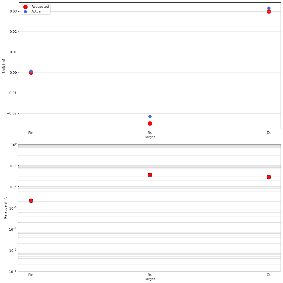
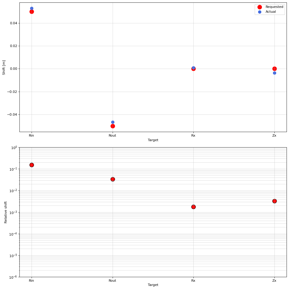
We can then measure the accuracy of the VCs by observing the difference between the requested change in shape targets vs. those enacted by the VCs.

for i in range(len(target_names)):
    print(f"Difference in {target_names[i]} = {np.round(new_target_values[i] - old_target_values[i],3)} vs. requested = {(requested_target_shifts)[i]}.")

Difference in Rin = 0.053 vs. requested = 0.05.
Difference in Rout = -0.046 vs. requested = -0.05.
Difference in Rx = 0.001 vs. requested = 0.0.
Difference in Zx = -0.004 vs. requested = 0.0.

In the plots below, we can see the actual shifts by the VCs are almost exactly as those requested (for the targets with actual shifts). Note how the unshifted targets also shift under the VCs due to the nonlinear coupling between targets and coil currents.

# plots
rel_diff = np.abs(np.array(new_target_values) - np.array(old_target_values))/np.abs(old_target_values)

fig1, ((ax1), (ax2)) = plt.subplots(2, 1, figsize=(12,12), dpi=80)

ax1.grid(True, which='both', alpha=0.5)
ax1.scatter(target_names, requested_target_shifts, color='red', marker='o', s=150, label="Requested")
ax1.scatter(target_names, np.array(new_target_values) - np.array(old_target_values), color='royalblue', marker='o', s=75, label="Actual")
ax1.set_xlabel("Target")
ax1.set_ylabel("Shift [m]")
ax1.legend()
# ax1.set_ylim([-max(targets_shift+non_standard_targets_shift)*1.1, max(targets_shift+non_standard_targets_shift)*1.1])

ax2.grid(True, which='both', alpha=0.5)
ax2.scatter(target_names, rel_diff, color='red', marker='o', s=150, edgecolors='black', label="Requested")
ax2.set_xlabel("Target")
ax2.set_ylabel("Relative shift")
labels = ax2.get_xticklabels()
ax2.set_yscale('log')
ax2.set_ylim([1e-6, 1e-0])

plt.tight_layout()

Alternative VCs

Note that when the VC_calculate method is called, a name can be provided. This will store the key data in a subclass with name. This useful for recalling from which targets and coils a given shape matrix or VC matrix was calculated.

Note that if no name is provided the default is used (“latest_VC”).

# display the attributes
print(VCs.VC_for_lower_targets.__dict__.keys())

dict_keys(['name', 'eq', 'profiles', 'shape_matrix', 'VCs_matrix', 'target_names', 'coils', 'target_calculator'])

You can then follow up by calculating alternative VCs for different target and coil combinations.

# define the descriptors function (it should return an array of values and take in an eq object)
def plasma_descriptors_new(eq):

    # inboard/outboard midplane radii
    RinRout = eq.innerOuterSeparatrix()

    # find lower X-point
    # define a "box" in which to search for the lower X-point
    XPT_BOX = [[0.33, -0.88], [0.95, -1.38]]

    # mask those points
    xpt_mask = (
        (eq.xpt[:, 0] >= XPT_BOX[0][0])
        & (eq.xpt[:, 0] <= XPT_BOX[1][0])
        & (eq.xpt[:, 1] <= XPT_BOX[0][1])
        & (eq.xpt[:, 1] >= XPT_BOX[1][1])
    )
    xpts = eq.xpt[xpt_mask, 0:2].squeeze()
    if xpts.ndim > 1 and xpts.shape[0] > 1:
        opt = eq.opt[0, 0:2]
        dists = np.linalg.norm(xpts - opt, axis=1)
        idx = np.argmin(dists)  # index of closest point
        Rx, Zx = xpts[idx, :]
    else:
        Rx, Zx = xpts

    return np.array([RinRout[0], Rx, Zx])

# this time we use only the divertor coils and a subset of targets
coils = ["PX", 'D1', 'D2', 'D3', 'Dp', 'D5', 'D6', 'D7']
target_names =['Rin', 'Rx', 'Zx']


# calculate the shape and VC matrices as follows
VCs.calculate_VC(
    eq=eq,
    profiles=profiles,
    coils=coils,
    target_names=target_names,
    target_calculator=plasma_descriptors_new,
    starting_dI=None,
    min_starting_dI=50,
    verbose=True,
    name="VC_for_upper_targets", # name for the VC
    )

--- Stage one ---
Re-sizing each initial coil current shift so that it produces a 0.1% change in plasma current density from the input equilibrium.
Forward static solve SUCCESS. Tolerance 1.13e-08 (vs. requested 1.00e-07) reached in 5/100 iterations.
Coil PX (original current shift = 50.0 [A] --> scaled current shift 27.05 [A]).

Forward static solve SUCCESS. Tolerance 9.21e-09 (vs. requested 1.00e-07) reached in 4/100 iterations.
Coil D1 (original current shift = 50.0 [A] --> scaled current shift 19.79 [A]).
Forward static solve SUCCESS. Tolerance 1.69e-08 (vs. requested 1.00e-07) reached in 3/100 iterations.
Coil D2 (original current shift = 50.0 [A] --> scaled current shift 20.14 [A]).
Forward static solve SUCCESS. Tolerance 7.47e-09 (vs. requested 1.00e-07) reached in 4/100 iterations.
Coil D3 (original current shift = 50.0 [A] --> scaled current shift 15.24 [A]).

Forward static solve SUCCESS. Tolerance 5.95e-08 (vs. requested 1.00e-07) reached in 4/100 iterations.
Coil Dp (original current shift = 50.0 [A] --> scaled current shift 6.41 [A]).
Forward static solve SUCCESS. Tolerance 1.40e-08 (vs. requested 1.00e-07) reached in 5/100 iterations.
Coil D5 (original current shift = 50.0 [A] --> scaled current shift 4.27 [A]).

Forward static solve SUCCESS. Tolerance 6.93e-09 (vs. requested 1.00e-07) reached in 4/100 iterations.
Coil D6 (original current shift = 50.0 [A] --> scaled current shift 4.4 [A]).
Forward static solve SUCCESS. Tolerance 3.75e-08 (vs. requested 1.00e-07) reached in 4/100 iterations.
Coil D7 (original current shift = 50.0 [A] --> scaled current shift 3.8 [A]).
--- Stage two ---
Building the shape matrix (Jacobian) of the shape parameter changes wrt scaled current shifts for each coil:
Coil PX

Forward static solve SUCCESS. Tolerance 6.83e-08 (vs. requested 1.00e-07) reached in 6/100 iterations.
Coil D1
Forward static solve SUCCESS. Tolerance 9.12e-08 (vs. requested 1.00e-07) reached in 3/100 iterations.
Coil D2
Forward static solve SUCCESS. Tolerance 8.09e-09 (vs. requested 1.00e-07) reached in 4/100 iterations.
Coil D3

Forward static solve SUCCESS. Tolerance 1.15e-08 (vs. requested 1.00e-07) reached in 3/100 iterations.
Coil Dp
Forward static solve SUCCESS. Tolerance 3.76e-08 (vs. requested 1.00e-07) reached in 3/100 iterations.
Coil D5
Forward static solve SUCCESS. Tolerance 2.60e-08 (vs. requested 1.00e-07) reached in 3/100 iterations.
Coil D6

Forward static solve SUCCESS. Tolerance 2.75e-08 (vs. requested 1.00e-07) reached in 3/100 iterations.
Coil D7
Forward static solve SUCCESS. Tolerance 1.32e-08 (vs. requested 1.00e-07) reached in 3/100 iterations.
--- Stage three ---
Inverting the shape matrix to get the virtual circuit matrix.
VC object stored under name: 'VC_for_upper_targets'.

# display the attributes
print(VCs.VC_for_upper_targets.__dict__.keys())

dict_keys(['name', 'eq', 'profiles', 'shape_matrix', 'VCs_matrix', 'target_names', 'coils', 'target_calculator'])

We can now apply this VC using the apply_VC method.

# we'll shift the upper strikepoint (R value) 
requested_target_shifts = [0.0, -0.025, 0.03]

# we apply the VCs to the some desired shifts, using the VC_object we just created
eq_new, profiles_new, new_target_values, old_target_values = VCs.apply_VC(
    eq=eq,
    profiles=profiles,
    VC_object=VCs.VC_for_upper_targets,
    requested_target_shifts=requested_target_shifts,
    verbose=True,
)

Currents shifts from VCs:
['PX', 'D1', 'D2', 'D3', 'Dp', 'D5', 'D6', 'D7'] = [1253.79306764  286.38800525    5.68112949  -58.52649482 -481.52918483
   92.30632864 -152.65025625   30.28339972].

Targets shifts from VCs:
['Rin', 'Rx', 'Zx'] = [ 0.00072327 -0.02149799  0.03151881].

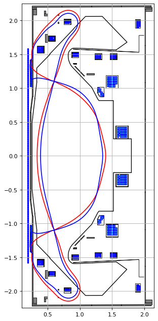
# plot the resulting equilbria 
fig1, ax1 = plt.subplots(1, 1, figsize=(4, 8), dpi=80)
ax1.grid(True, which='both')
ax1.plot(eq.tokamak.wall.R, eq.tokamak.wall.Z, color='k', linewidth=1.2, linestyle="-")
eq.tokamak.plot(axis=ax1, show=False)

ax1.contour(eq.R, eq.Z, eq.psi(), levels=[eq.psi_bndry], colors='r')
ax1.contour(eq.R, eq.Z, eq_new.psi(), levels=[eq_new.psi_bndry], colors='b')

ax1.set_xlim(0.1, 2.15)
ax1.set_ylim(-2.25, 2.25)

plt.tight_layout()

# plots
rel_diff = np.abs(np.array(new_target_values) - np.array(old_target_values))/np.abs(old_target_values)

fig1, ((ax1), (ax2)) = plt.subplots(2, 1, figsize=(12,12), dpi=80)

ax1.grid(True, which='both', alpha=0.5)
ax1.scatter(target_names, requested_target_shifts, color='red', marker='o', s=150, label="Requested")
ax1.scatter(target_names, np.array(new_target_values) - np.array(old_target_values), color='royalblue', marker='o', s=75, label="Actual")
ax1.set_xlabel("Target")
ax1.set_ylabel("Shift [m]")
ax1.legend()
# ax1.set_ylim([-max(targets_shift+non_standard_targets_shift)*1.1, max(targets_shift+non_standard_targets_shift)*1.1])

ax2.grid(True, which='both', alpha=0.5)
ax2.scatter(target_names, rel_diff, color='red', marker='o', s=150, edgecolors='black', label="Requested")
ax2.set_xlabel("Target")
ax2.set_ylabel("Relative shift")
labels = ax2.get_xticklabels()
ax2.set_yscale('log')
ax2.set_ylim([1e-6, 1e-0])

plt.tight_layout()