Example: Obtaining results from the eq and profiles objects
Here we will take a look at how to access different results stored (or calculated using methods) in the eq and profiles objects.
To do this we first need to run a static forward simulation in the MAST-U-like tokamak using previously saved coil currents to generate our results. Of course, the same methods below can be applied after an inverse solve!
Static forward simulation
import matplotlib.pyplot as plt
import numpy as np
# build machine
from freegsnke import build_machine
tokamak = build_machine.tokamak(
active_coils_path=f"../machine_configs/MAST-U/MAST-U_like_active_coils.pickle",
passive_coils_path=f"../machine_configs/MAST-U/MAST-U_like_passive_coils.pickle",
limiter_path=f"../machine_configs/MAST-U/MAST-U_like_limiter.pickle",
wall_path=f"../machine_configs/MAST-U/MAST-U_like_wall.pickle",
)
# initialise equilibrium object
from freegsnke import equilibrium_update
eq = equilibrium_update.Equilibrium(
tokamak=tokamak,
Rmin=0.1, Rmax=2.0, # radial range
Zmin=-2.2, Zmax=2.2, # vertical range
nx=65, # number of grid points in the radial direction (needs to be of the form (2**n + 1) with n being an integer)
ny=129, # number of grid points in the vertical direction (needs to be of the form (2**n + 1) with n being an integer)
# psi=plasma_psi
)
# initialise profile object
from freegsnke.jtor_update import ConstrainPaxisIp
profiles = ConstrainPaxisIp(
eq=eq,
paxis=8.1e3,
Ip=6.2e5,
fvac=0.5,
alpha_m=1.8,
alpha_n=1.2
)
# initialise solver
from freegsnke import GSstaticsolver
GSStaticSolver = GSstaticsolver.NKGSsolver(eq)
# set coil currents
import pickle
with open('simple_diverted_currents_PaxisIp.pk', 'rb') as f:
current_values = pickle.load(f)
for key in current_values.keys():
eq.tokamak[key].current = current_values[key]
# carry out forward solve
GSStaticSolver.solve(eq=eq,
profiles=profiles,
constrain=None,
target_relative_tolerance=1e-9)
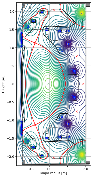
# plot the resulting equilbrium
fig1, ax1 = plt.subplots(1, 1, figsize=(4, 8), dpi=80)
ax1.grid(True, which='both')
eq.plot(axis=ax1, show=False)
eq.tokamak.plot(axis=ax1, show=False)
ax1.set_xlim(0.1, 2.15)
ax1.set_ylim(-2.25, 2.25)
plt.tight_layout()
Active coils --> built from pickle file.
Passive structures --> built from pickle file.
Limiter --> built from pickle file.
Wall --> built from pickle file.
Magnetic probes --> none provided.
Resistance (R) and inductance (M) matrices --> built using actives (and passives if present).
Tokamak built.
Forward static solve SUCCESS. Tolerance 8.07e-10 (vs. requested 1.00e-09) reached in 26/100 iterations.
Dashboard of results
It is worth playing around with the fields/methods in the eq and profiles objects yourself to see which quantities can be calculated from the plasma equilibrium using built-in functionality. Below, we provide a mini dashboard of different quantities and how to generate them.
If there are certain quantites that you wish to be added that don’t exist within FreeGSNKE at the moment, please do submit a feature request to the Github repository.
General equillibrium quantites
Here, we display a number of used equilibrium quantites.
# plasma quantities
print(rf"Plasma current: {eq.plasmaCurrent()} [A]")
print("---")
print(rf"Poloidal beta (definition 1): {eq.poloidalBeta()}")
print(rf"Poloidal beta (definition 2): {eq.poloidalBeta2()}")
print(rf"Toroidal beta: {eq.toroidalBeta()}")
print(rf"Normalised total beta: {eq.normalised_total_Beta()}")
print("---")
print(fr"Plasma internal inductance (li1): {eq.internalInductance1()}")
print(fr"Plasma internal inductance (li2): {eq.internalInductance2()}")
print(fr"Plasma internal inductance (li3): {eq.internalInductance3()}")
Plasma current: 620000.0 [A]
---
Dicrepancy between psi_func and plasma_psi detected. psi_func has been re-set.
Poloidal beta (definition 1): 0.18994413047198333
Poloidal beta (definition 2): 0.27694693475312154
Toroidal beta: 0.014584893020785562
Normalised total beta: 0.013855233051745304
---
Plasma internal inductance (li1): 2.2793698999635787
Plasma internal inductance (li2): 0.6546157216633977
Plasma internal inductance (li3): 0.7114630299114697
# plasma geometry quantities
print(rf"Minor radius: {eq.minorRadius()} [m]")
print("---")
print(rf"Magnetic axis location: {eq.magneticAxis()[0:2]} [m]")
print(rf"Geometric axis location: {eq.geometricAxis()} [m]")
print(rf"Shafranov shift: {eq.shafranov_shift()} [m]")
print(rf"Inner and outer mipdplane (Z=0) radii: {eq.innerOuterSeparatrix(Z=0)} [m]")
print(rf"Inner and outer mipdplane (Z=0) radii (alternative): {eq.innerOuterSeparatrix2(Z=0)} [m]")

print("---")
print(rf"LCFS circumference: {eq.separatrix_length()} [m]")
print(rf"LCFS area: {eq.separatrix_area()} [m^2]")
print(rf"Plasma volume: {eq.plasmaVolume()} [m^3]")

print("---")
print(rf"Aspect ratio: {eq.aspectRatio()}")

print("---")
print(rf"Geometric elongation: {eq.geometricElongation()}")
print(rf"Geometric elongation (upper): {eq.geometricElongation_upper()}")
print(rf"Geometric elongation (lower): {eq.geometricElongation_lower()}")
print(rf"Effective elongation: {eq.effectiveElongation()}")

print("---")
print(rf"Triangularity: {eq.triangularity()}")
print(rf"Triangularity (upper): {eq.triangularity_upper()}")
print(rf"Triangularity (lower): {eq.triangularity_lower()}")

print("---")
s_uo, s_ui, s_lo, s_li = eq.squareness()
print(rf"Squareness (upper outer): {s_uo}")
print(rf"Squareness (upper inner): {s_ui}")
print(rf"Squareness (lower outer): {s_lo}")
print(rf"Squareness (lower inner): {s_li}")

print("---")
L = eq.closest_wall_point()
print(rf"Point on wall that is closest to the LCFS: {L[0]} [m]")
print(rf"Corresponding distance from point to LCFS: {L[1]} [m]")

print("---")
print(rf"Is this a limited plasma?: {eq.flag_limiter}")
print(rf"Does the core plasma boundary intersect the wall?: {eq.intersectsWall()}")
Minor radius: 0.5470006855894912 [m]
---
Magnetic axis location: [ 9.77402539e-01 -5.07484561e-08] [m]
Geometric axis location: [ 8.99306137e-01 -1.22824229e-08] [m]
Shafranov shift: [ 7.80964029e-02 -3.84660333e-08] [m]
Inner and outer mipdplane (Z=0) radii: (0.3519521633313429, 1.4464481306863588) [m]
Inner and outer mipdplane (Z=0) radii (alternative): [(0.3523054510727558, 0.0), (1.4463068216936634, 0.0)] [m]
---
LCFS circumference: 7.857641901226211 [m]
LCFS area: 1.7493546389888184 [m^2]
Plasma volume: 9.234156383614367 [m^3]
---
Aspect ratio: 1.6440676588510614
---
Geometric elongation: 3.18430227822949
Geometric elongation (upper): 3.1843023485512183
Geometric elongation (lower): 3.1843022079077614
Effective elongation: 1.738537992960958
---
Triangularity: 0.8918704905059383
Triangularity (upper): 0.8918704676570228
Triangularity (lower): 0.8918705133548536
---
Squareness (upper outer): -0.5962390003909828
Squareness (upper inner): 0.5919119319583072
Squareness (lower outer): -0.5962390145353256
Squareness (lower inner): 0.5919119351821343
---
Point on wall that is closest to the LCFS: [0.50148    1.49122494] [m]
Corresponding distance from point to LCFS: 0.034412608520673606 [m]
---
Is this a limited plasma?: False
Does the core plasma boundary intersect the wall?: True
print(rf"Aspect ratio: {eq.aspectRatio()}")
print(rf"Geometric elongation: {eq.geometricElongation()}")
print(rf"Effective elongation: {eq.effectiveElongation()}")
print(rf"Poloidal beta (method 1): {eq.poloidalBeta()}")
print(rf"Poloidal beta (method 2): {eq.poloidalBeta2()}")
print(rf"Toroidal beta: {eq.toroidalBeta()}")
print(rf"Normalised total plasma beta: {eq.normalised_total_Beta()}")
print(rf"Plasma volume: {eq.plasmaVolume()}")
Aspect ratio: 1.6440676588510614
Geometric elongation: 3.18430227822949
Effective elongation: 1.738537992960958
Poloidal beta (method 1): 0.18994413047198333
Poloidal beta (method 2): 0.27694693475312154
Toroidal beta: 0.014584893020785562
Normalised total plasma beta: 0.013855233051745304
Plasma volume: 9.234156383614367
print(fr"Poloidal flux on magnetic axis: {eq.psi_axis} [Webers/2\pi]")
print(fr"Poloidal flux on plasma boundary: {eq.psi_bndry} [Webers/2\pi]")
Poloidal flux on magnetic axis: 0.09806848634906881 [Webers/2\pi]
Poloidal flux on plasma boundary: 0.030325899245174037 [Webers/2\pi]
# extract the plasma core boundary (specify the number of points you want)
eq.separatrix(ntheta=20)
array([[ 9.77402539e-01,  9.15865074e-01],
       [ 1.20450668e+00,  6.98954611e-01],
       [ 1.32854569e+00,  4.83307034e-01],
       [ 1.38398966e+00,  2.95402780e-01],
       [ 1.42598741e+00,  1.45754008e-01],
       [ 1.44630682e+00, -5.07484565e-08],
       [ 1.42598739e+00, -1.45754105e-01],
       [ 1.38398965e+00, -2.95402877e-01],
       [ 1.32854569e+00, -4.83307138e-01],
       [ 1.20450667e+00, -6.98954696e-01],
       [ 9.77402539e-01, -9.15865179e-01],
       [ 4.11452379e-01, -1.74181554e+00],
       [ 4.62740252e-01, -7.08371918e-01],
       [ 3.91352872e-01, -4.25790058e-01],
       [ 3.60736194e-01, -2.00367092e-01],
       [ 3.52305451e-01, -5.07484566e-08],
       [ 3.60736197e-01,  2.00366990e-01],
       [ 3.91352879e-01,  4.25789951e-01],
       [ 4.62740272e-01,  7.08371789e-01],
       [ 4.11452354e-01,  1.74181552e+00]])
# extract the X points (R, Z, psi)
eq.xpt
array([[ 6.12921154e-01, -1.12680620e+00,  3.03258992e-02],
       [ 6.12921156e-01,  1.12680612e+00,  3.03258959e-02],
       [ 1.12149912e+00, -2.04026719e+00,  2.76630384e-02],
       [ 1.12149912e+00,  2.04026719e+00,  2.76630376e-02],
       [ 1.75924847e+00, -7.59569056e-01, -2.06708051e-02],
       [ 1.75924846e+00,  7.59569059e-01, -2.06708071e-02],
       [ 1.93437406e+00, -1.27780331e-08, -2.09893282e-02]])
# extract the strike points where the separatric intersects the wall, if any (R, Z)
eq.strikepoints()
array([[ 1.70945878, -1.66697042],
       [ 1.30726323, -2.06534044],
       [ 1.30869545,  2.06026479],
       [ 1.71263706,  1.66516759],
       [ 0.95834741, -1.93862429],
       [ 0.9569785 ,  1.92974657],
       [ 0.332797  ,  1.25443764],
       [ 0.332797  , -1.25443759]])
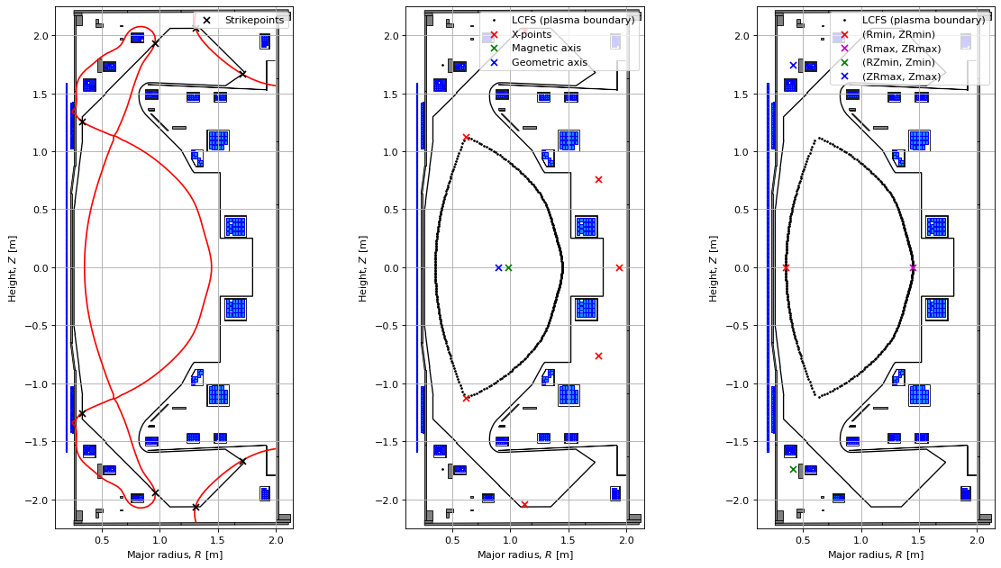
# here we plot some of the features above on different axes to show where they are located (see code documentation for more details)

sep = eq.separatrix(ntheta=360)
strikes = eq.strikepoints()

fig1, (ax1, ax2, ax3) = plt.subplots(1, 3, figsize=(15, 8), dpi=80)
plt.subplots_adjust(wspace=0.25)  # adjust the horizontal space between subplots

ax1.grid(True, which='both')
eq.tokamak.plot(axis=ax1,show=False)
ax1.fill(tokamak.wall.R, tokamak.wall.Z, color='k', linewidth=1.2, facecolor='w', zorder=0)
ax1.contour(eq.R, eq.Z, eq.psi(), levels=[eq.psi_bndry], linestyles='solid', colors='r') #, label="Separatrix")
ax1.scatter(strikes[:,0], strikes[:,1], color='k', marker='x', s=40, zorder=2, label="Strikepoints")
ax1.set_aspect('equal')
ax1.set_xlim(0.1, 2.15)
ax1.set_ylim(-2.25, 2.25)
ax1.set_xlabel(r'Major radius, $R$ [m]')
ax1.set_ylabel(r'Height, $Z$ [m]')
ax1.legend(loc="upper right")


ax2.grid(True, which='both')
eq.tokamak.plot(axis=ax2,show=False)
ax2.fill(tokamak.wall.R, tokamak.wall.Z, color='k', linewidth=1.2, facecolor='w', zorder=0)
ax2.scatter(sep[:,0], sep[:,1], color='k', marker='o', s=2, zorder=2, label="LCFS (plasma boundary)")
ax2.scatter(eq.xpt[:,0], eq.xpt[:,1], color='r', marker='x', s=40, zorder=2, label="X-points")
ax2.scatter(eq.magneticAxis()[0], eq.magneticAxis()[1], color='g', marker='x', s=40, zorder=2, label="Magnetic axis")
ax2.scatter(eq.geometricAxis()[0], eq.geometricAxis()[1], color='b', marker='x', s=40, zorder=2, label="Geometric axis")
ax2.set_aspect('equal')
ax2.set_xlim(0.1, 2.15)
ax2.set_ylim(-2.25, 2.25)
ax2.set_xlabel(r'Major radius, $R$ [m]')
ax2.set_ylabel(r'Height, $Z$ [m]')
ax2.legend(loc="upper right")


ax3.grid(True, which='both')
eq.tokamak.plot(axis=ax3,show=False)
ax3.fill(tokamak.wall.R, tokamak.wall.Z, color='k', linewidth=1.2, facecolor='w', zorder=0)
ax3.scatter(sep[:,0], sep[:,1], color='k', marker='o', s=2, zorder=2, label="LCFS (plasma boundary)")
ax3.scatter(eq._sep_Rmin, eq._sep_ZRmin, color='r', marker='x', s=40, zorder=2, label="(Rmin, ZRmin)")
ax3.scatter(eq._sep_Rmax, eq._sep_ZRmax, color='m', marker='x', s=40, zorder=2, label="(Rmax, ZRmax)")
ax3.scatter(eq._sep_RZmin, eq._sep_Zmin, color='g', marker='x', s=40, zorder=2, label="(RZmin, Zmin)")
ax3.scatter(eq._sep_RZmax, eq._sep_Zmax, color='b', marker='x', s=40, zorder=2, label="(ZRmax, Zmax)")
ax3.set_aspect('equal')
ax3.set_xlim(0.1, 2.15)
ax3.set_ylim(-2.25, 2.25)
ax3.set_xlabel(r'Major radius, $R$ [m]')
ax3.set_ylabel(r'Height, $Z$ [m]')
ax3.legend(loc="upper right")

plt.tight_layout()
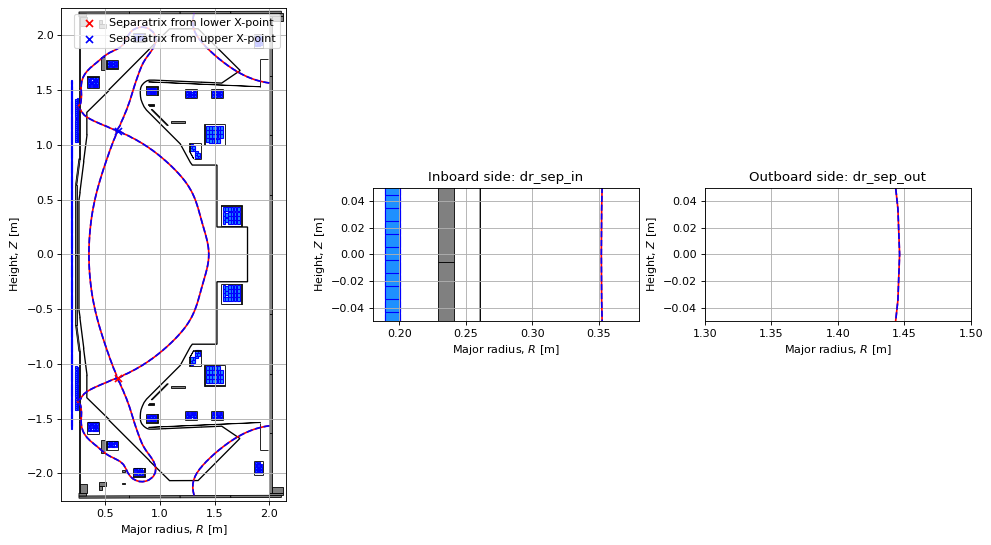
Here we visualise the dr sep quantities.
This two distances are defined as the radial separation (on the inboard and outboard sides) at the midplane (Z = 0) between flux surfaces passing through the lower and upper X-points.
dr_seps = eq.dr_sep()

print(f"dr_sep_in = {dr_seps[0]} [m].")
print(f"dr_sep_out = {dr_seps[1]} [m].")
dr_sep_in = 3.1670866762478767e-08 [m].
dr_sep_out = -1.5165753763923817e-08 [m].
In the plot below, dr_sep_in is the difference between the radial position of the blue and the red flux surfaces at \(Z=0\).
Similarly, dr_sep_out is the difference between the radial position of the red and the blue flux surfaces at \(Z=0\).
# visualising these quantities
psi_bndry = eq.psi_bndry
xpts = eq.xpt

# compute absolute difference between each point's ψ and psi_bndry and then
# get indices of the two smallest differences
closest_indices = np.argsort(np.abs(xpts[:, 2] - psi_bndry))[:2]

# extract the corresponding rows (two X-points closest to psi_bndry, then sort by lowest z coord z-point)
closest_xpts = xpts[closest_indices]
closest_xpts_sorted = closest_xpts[np.argsort(closest_xpts[:, 1])]

# plot the flux contours for the values of psi_boundary at each X-point
fig1, axes = plt.subplots(1, 3, figsize=(15, 8), dpi=80)
plt.subplots_adjust(wspace=0.25)  # adjust the horizontal space between subplots

axes[0].grid(True, which='both')
eq.tokamak.plot(axis=axes[0],show=False)
axes[0].fill(tokamak.wall.R, tokamak.wall.Z, color='k', linewidth=1.2, facecolor='w', zorder=0)
axes[0].contour(eq.R, eq.Z, eq.psi(), levels=[closest_xpts_sorted[0, 2]], linestyles='solid', colors='r')
axes[0].contour(eq.R, eq.Z, eq.psi(), levels=[closest_xpts_sorted[1, 2]], linestyles='dashed', colors='b')
axes[0].scatter(closest_xpts_sorted[0,0], closest_xpts_sorted[0,1], color='r', marker='x', s=40, zorder=2, label="Separatrix from lower X-point")
axes[0].scatter(closest_xpts_sorted[1,0], closest_xpts_sorted[1,1], color='b', marker='x', s=40, zorder=2, label="Separatrix from upper X-point")
axes[0].set_aspect('equal')
axes[0].set_xlim(0.1, 2.15)
axes[0].set_ylim(-2.25, 2.25)
axes[0].set_xlabel(r'Major radius, $R$ [m]')
axes[0].set_ylabel(r'Height, $Z$ [m]')
axes[0].legend(loc="upper right")


axes[1].grid(True, which='both')
eq.tokamak.plot(axis=axes[1],show=False)
axes[1].fill(tokamak.wall.R, tokamak.wall.Z, color='k', linewidth=1.2, facecolor='w', zorder=0)
axes[1].contour(eq.R, eq.Z, eq.psi(), levels=[closest_xpts_sorted[0, 2]], linestyles='solid', colors='r')
axes[1].contour(eq.R, eq.Z, eq.psi(), levels=[closest_xpts_sorted[1, 2]], linestyles='dashed', colors='b')
axes[1].scatter(closest_xpts_sorted[0,0], closest_xpts_sorted[0,1], color='r', marker='x', s=40, zorder=2, label="Separatrix from lower X-point")
axes[1].scatter(closest_xpts_sorted[1,0], closest_xpts_sorted[1,1], color='b', marker='x', s=40, zorder=2, label="Separatrix from upper X-point")
axes[1].set_aspect('equal')
axes[1].set_xlim(0.18, 0.38)
axes[1].set_ylim(-0.05, 0.05)
axes[1].set_xlabel(r'Major radius, $R$ [m]')
axes[1].set_ylabel(r'Height, $Z$ [m]')
axes[1].set_title("Inboard side: dr_sep_in")


axes[2].grid(True, which='both')
eq.tokamak.plot(axis=axes[2],show=False)
axes[2].fill(tokamak.wall.R, tokamak.wall.Z, color='k', linewidth=1.2, facecolor='w', zorder=0)
axes[2].contour(eq.R, eq.Z, eq.psi(), levels=[closest_xpts_sorted[0, 2]], linestyles='solid', colors='r')
axes[2].contour(eq.R, eq.Z, eq.psi(), levels=[closest_xpts_sorted[1, 2]], linestyles='dashed', colors='b')
axes[2].scatter(closest_xpts_sorted[0,0], closest_xpts_sorted[0,1], color='r', marker='x', s=40, zorder=2, label="Separatrix from lower X-point")
axes[2].scatter(closest_xpts_sorted[1,0], closest_xpts_sorted[1,1], color='b', marker='x', s=40, zorder=2, label="Separatrix from upper X-point")
axes[2].set_aspect('equal')
axes[2].set_xlim(1.3, 1.5)
axes[2].set_ylim(-0.05, 0.05)
axes[2].set_xlabel(r'Major radius, $R$ [m]')
axes[2].set_ylabel(r'Height, $Z$ [m]')
axes[2].set_title("Outboard side: dr_sep_out")
Text(0.5, 1.0, 'Outboard side: dr_sep_out')
Flux quantites
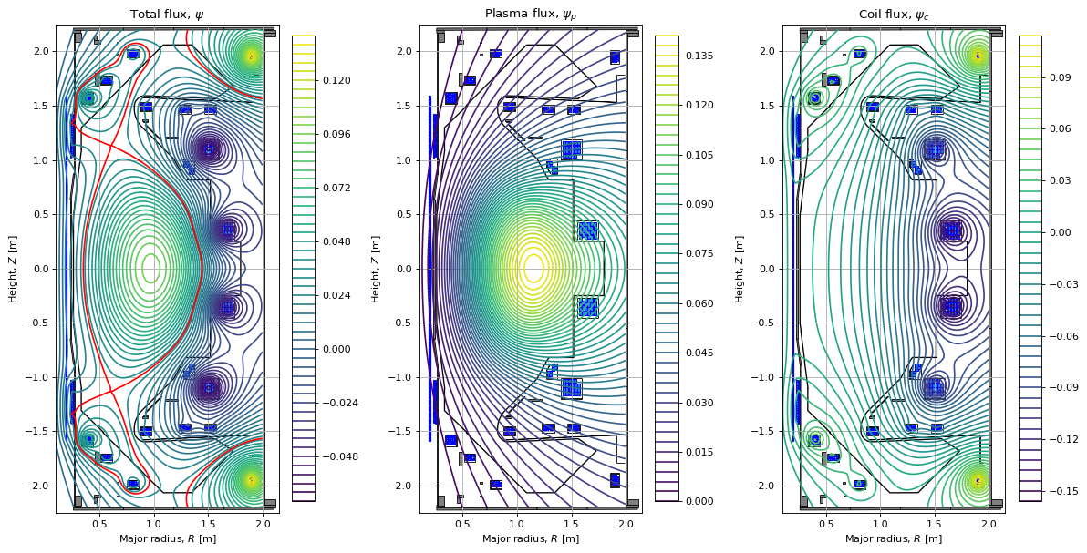
Here, we plot the total poloidal flux \(\psi\) [Webers / \(2\pi\)] and its two components \(\psi_p\) (the plasma flux) and \(\psi_c\) (the coil flux): \(\psi = \psi_p + \psi_c\).
fig1, (ax1, ax2, ax3) = plt.subplots(1, 3, figsize=(15, 8), dpi=80)
plt.subplots_adjust(wspace=0.5)  # adjust the horizontal space between subplots

ax1.grid(True, which='both')
eq.tokamak.plot(axis=ax1,show=False)
# ax1.plot(tokamak.limiter.R, tokamak.limiter.Z, color='k', linewidth=1.2, linestyle="--")
ax1.plot(tokamak.wall.R, tokamak.wall.Z, color='k', linewidth=1.2, linestyle="-")
im1 = ax1.contour(eq.R, eq.Z, eq.psi(), levels=50)                          # total psi
ax1.contour(eq.R, eq.Z, eq.psi(), levels=[eq.psi_bndry], colors='r')  # psi boundary contour
ax1.set_aspect('equal')
ax1.set_xlim(0.1, 2.15)
ax1.set_ylim(-2.25, 2.25)
ax1.set_title(r"Total flux, $\psi$")
ax1.set_xlabel(r'Major radius, $R$ [m]')
ax1.set_ylabel(r'Height, $Z$ [m]')
cbar = plt.colorbar(im1, ax=ax1, fraction=0.09)


ax2.grid(True, which='both')
eq.tokamak.plot(axis=ax2,show=False)
# ax2.plot(tokamak.limiter.R, tokamak.limiter.Z, color='k', linewidth=1.2, linestyle="--")
ax2.plot(tokamak.wall.R, tokamak.wall.Z, color='k', linewidth=1.2, linestyle="-")
im2 = ax2.contour(eq.R, eq.Z, eq.plasma_psi, levels=50)                          # plasma psi
ax2.set_aspect('equal')
ax2.set_xlim(0.1, 2.15)
ax2.set_ylim(-2.25, 2.25)
ax2.set_title(r"Plasma flux, $\psi_p$")
ax2.set_xlabel(r'Major radius, $R$ [m]')
ax2.set_ylabel(r'Height, $Z$ [m]')
cbar = plt.colorbar(im2, ax=ax2, fraction=0.09)


ax3.grid(True, which='both')
eq.tokamak.plot(axis=ax3,show=False)
# ax3.plot(tokamak.limiter.R, tokamak.limiter.Z, color='k', linewidth=1.2, linestyle="--")
ax3.plot(tokamak.wall.R, tokamak.wall.Z, color='k', linewidth=1.2, linestyle="-")
im3 = ax3.contour(eq.R, eq.Z, eq.tokamak_psi, levels=50)                          # coil psi
ax3.set_aspect('equal')
ax3.set_xlim(0.1, 2.15)
ax3.set_ylim(-2.25, 2.25)
ax3.set_title(r"Coil flux, $\psi_c$")
ax3.set_xlabel(r'Major radius, $R$ [m]')
ax3.set_ylabel(r'Height, $Z$ [m]')
cbar = plt.colorbar(im3, ax=ax3, fraction=0.09)


plt.tight_layout()
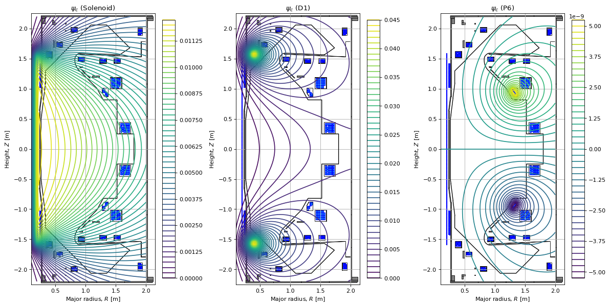
We can also extract the flux produced by individual coils (or pasive structures) if required. We do this my using the pre-calculated Green’s functions, the coil currents, multipliers, and polarities.
currents = eq.tokamak.getCurrents()

# calculate the active/passive coil fluxes

psi_coils = dict()
for i, name in enumerate(currents.keys()):
    coil = eq.tokamak.coils_dict[name]
    scaling = coil["multiplier"]*coil["polarity"]
    greens_matrix = 0.0

    if type(eq._pgreen[name]) is dict:
        num_coils = len(eq._pgreen[name])
        for i, ind in enumerate(eq._pgreen[name]):
            greens_matrix += eq._pgreen[name][ind]*scaling[i*(len(scaling)//num_coils)]
    else:
        num_coils = 1
        greens_matrix = eq._pgreen[name]*scaling[0]

    psi_coils[name] = greens_matrix*currents[name]
Here, we plot a few of the fluxes from the coils. You can change the name parameters to visualise different coil fluxes.
fig1, (ax1, ax2, ax3) = plt.subplots(1, 3, figsize=(15, 8), dpi=80)
plt.subplots_adjust(wspace=0.5)  # adjust the horizontal space between subplots

name = "Solenoid"
ax1.grid(True, which='both')
eq.tokamak.plot(axis=ax1,show=False)
# ax1.plot(tokamak.limiter.R, tokamak.limiter.Z, color='k', linewidth=1.2, linestyle="--")
ax1.plot(tokamak.wall.R, tokamak.wall.Z, color='k', linewidth=1.2, linestyle="-")
im1 = ax1.contour(eq.R, eq.Z, psi_coils[name], levels=50)
ax1.set_aspect('equal')
ax1.set_xlim(0.1, 2.15)
ax1.set_ylim(-2.25, 2.25)
ax1.set_title(rf"$\psi_c$ ({name})")
ax1.set_xlabel(r'Major radius, $R$ [m]')
ax1.set_ylabel(r'Height, $Z$ [m]')
cbar = plt.colorbar(im1, ax=ax1, fraction=0.09)

name = "D1"
ax2.grid(True, which='both')
eq.tokamak.plot(axis=ax2,show=False)
# ax2.plot(tokamak.limiter.R, tokamak.limiter.Z, color='k', linewidth=1.2, linestyle="--")
ax2.plot(tokamak.wall.R, tokamak.wall.Z, color='k', linewidth=1.2, linestyle="-")
im2 = ax2.contour(eq.R, eq.Z, psi_coils[name], levels=50)
ax2.set_aspect('equal')
ax2.set_xlim(0.1, 2.15)
ax2.set_ylim(-2.25, 2.25)
ax2.set_title(rf"$\psi_c$ ({name})")
ax2.set_xlabel(r'Major radius, $R$ [m]')
ax2.set_ylabel(r'Height, $Z$ [m]')
cbar = plt.colorbar(im2, ax=ax2, fraction=0.09)

name = "P6"
ax3.grid(True, which='both')
eq.tokamak.plot(axis=ax3,show=False)
# ax3.plot(tokamak.limiter.R, tokamak.limiter.Z, color='k', linewidth=1.2, linestyle="--")
ax3.plot(tokamak.wall.R, tokamak.wall.Z, color='k', linewidth=1.2, linestyle="-")
im3 = ax3.contour(eq.R, eq.Z, psi_coils[name], levels=50)
ax3.set_aspect('equal')
ax3.set_xlim(0.1, 2.15)
ax3.set_ylim(-2.25, 2.25)
ax3.set_title(rf"$\psi_c$ ({name})")
ax3.set_xlabel(r'Major radius, $R$ [m]')
ax3.set_ylabel(r'Height, $Z$ [m]')
cbar = plt.colorbar(im3, ax=ax3, fraction=0.09)


plt.tight_layout()
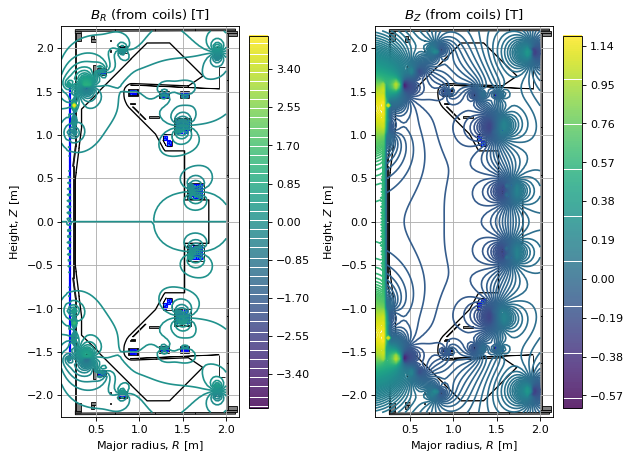
Magnetic fields
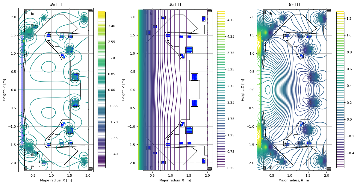
Here, we plot the different magnetic field components over the domain.
fig1, (ax1, ax2, ax3) = plt.subplots(1, 3, figsize=(15, 8), dpi=80)
plt.subplots_adjust(wspace=0.5)  # adjust the horizontal space between subplots

ax1.grid(True, which='both')
eq.tokamak.plot(axis=ax1,show=False)
# ax1.plot(tokamak.limiter.R, tokamak.limiter.Z, color='k', linewidth=1.2, linestyle="--")
ax1.plot(tokamak.wall.R, tokamak.wall.Z, color='k', linewidth=1.2, linestyle="-")
im1 = ax1.contour(eq.R, eq.Z, eq.Br(eq.R, eq.Z), levels=200)
ax1.set_aspect('equal')
ax1.set_xlim(0.1, 2.15)
ax1.set_ylim(-2.25, 2.25)
ax1.set_title(r"$B_R$ [T]")
ax1.set_xlabel(r'Major radius, $R$ [m]')
ax1.set_ylabel(r'Height, $Z$ [m]')
cbar = plt.colorbar(im1, ax=ax1, fraction=0.09)


ax2.grid(True, which='both')
eq.tokamak.plot(axis=ax2,show=False)
# ax2.plot(tokamak.limiter.R, tokamak.limiter.Z, color='k', linewidth=1.2, linestyle="--")
ax2.plot(tokamak.wall.R, tokamak.wall.Z, color='k', linewidth=1.2, linestyle="-")
im2 = ax2.contour(eq.R, eq.Z, eq.Btor(eq.R, eq.Z), levels=100)
ax2.set_aspect('equal')
ax2.set_xlim(0.1, 2.15)
ax2.set_ylim(-2.25, 2.25)
ax2.set_title(r"$B_{\phi}$ [T]")
ax2.set_xlabel(r'Major radius, $R$ [m]')
ax2.set_ylabel(r'Height, $Z$ [m]')
cbar = plt.colorbar(im2, ax=ax2, fraction=0.09)


ax3.grid(True, which='both')
eq.tokamak.plot(axis=ax3,show=False)
# ax3.plot(tokamak.limiter.R, tokamak.limiter.Z, color='k', linewidth=1.2, linestyle="--")
ax3.plot(tokamak.wall.R, tokamak.wall.Z, color='k', linewidth=1.2, linestyle="-")
im3 = ax3.contour(eq.R, eq.Z, eq.Bz(eq.R, eq.Z), levels=100)
ax3.set_aspect('equal')
ax3.set_xlim(0.1, 2.15)
ax3.set_ylim(-2.25, 2.25)
ax3.set_title(r"$B_Z$ [T]")
ax3.set_xlabel(r'Major radius, $R$ [m]')
ax3.set_ylabel(r'Height, $Z$ [m]')
cbar = plt.colorbar(im3, ax=ax3, fraction=0.09)


plt.tight_layout()
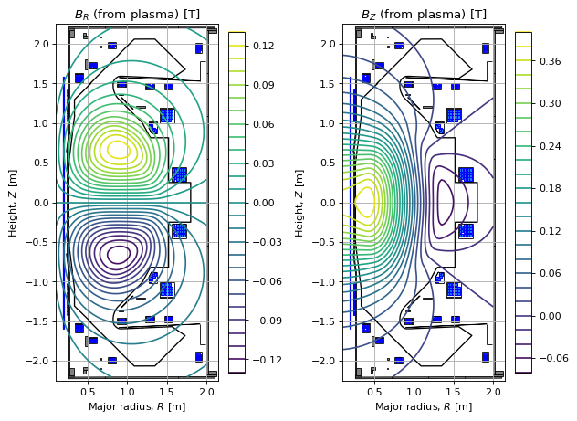
# this is just the contribution from the plasma
fig1, (ax1, ax2) = plt.subplots(1, 2, figsize=(8, 8), dpi=80)
plt.subplots_adjust(wspace=0.5)  # adjust the horizontal space between subplots

ax1.grid(True, which='both')
eq.tokamak.plot(axis=ax1,show=False)
# ax1.plot(tokamak.limiter.R, tokamak.limiter.Z, color='k', linewidth=1.2, linestyle="--")
ax1.plot(tokamak.wall.R, tokamak.wall.Z, color='k', linewidth=1.2, linestyle="-")
im1 = ax1.contour(eq.R, eq.Z, eq.plasmaBr(eq.R, eq.Z), levels=30)
ax1.set_aspect('equal')
ax1.set_xlim(0.1, 2.15)
ax1.set_ylim(-2.25, 2.25)
ax1.set_title(r"$B_R$ (from plasma) [T]")
ax1.set_xlabel(r'Major radius, $R$ [m]')
ax1.set_ylabel(r'Height, $Z$ [m]')
cbar = plt.colorbar(im1, ax=ax1, fraction=0.09)


ax2.grid(True, which='both')
eq.tokamak.plot(axis=ax2,show=False)
# ax2.plot(tokamak.limiter.R, tokamak.limiter.Z, color='k', linewidth=1.2, linestyle="--")
ax2.plot(tokamak.wall.R, tokamak.wall.Z, color='k', linewidth=1.2, linestyle="-")
im2 = ax2.contour(eq.R, eq.Z, eq.plasmaBz(eq.R, eq.Z), levels=30)
ax2.set_aspect('equal')
ax2.set_xlim(0.1, 2.15)
ax2.set_ylim(-2.25, 2.25)
ax2.set_title(r"$B_Z$ (from plasma) [T]")
ax2.set_xlabel(r'Major radius, $R$ [m]')
ax2.set_ylabel(r'Height, $Z$ [m]')
cbar = plt.colorbar(im2, ax=ax2, fraction=0.09)


plt.tight_layout()
# this is just the contribution from the active coils

Br_actives = 0.0
Bz_actives = 0.0
for name in eq.tokamak.coils_list[0:12]:
    Br_actives += eq.tokamak[name].Br(eq.R, eq.Z)
    Bz_actives += eq.tokamak[name].Bz(eq.R, eq.Z)

fig1, (ax1, ax2) = plt.subplots(1, 2, figsize=(8, 8), dpi=80)
plt.subplots_adjust(wspace=0.5)  # adjust the horizontal space between subplots

ax1.grid(True, which='both')
eq.tokamak.plot(axis=ax1,show=False)
# ax1.plot(tokamak.limiter.R, tokamak.limiter.Z, color='k', linewidth=1.2, linestyle="--")
ax1.plot(tokamak.wall.R, tokamak.wall.Z, color='k', linewidth=1.2, linestyle="-")
im1 = ax1.contour(eq.R, eq.Z, Br_actives, levels=200)
ax1.set_aspect('equal')
ax1.set_xlim(0.1, 2.15)
ax1.set_ylim(-2.25, 2.25)
ax1.set_title(r"$B_R$ (from coils) [T]")
ax1.set_xlabel(r'Major radius, $R$ [m]')
ax1.set_ylabel(r'Height, $Z$ [m]')
cbar = plt.colorbar(im1, ax=ax1, fraction=0.09)


ax2.grid(True, which='both')
eq.tokamak.plot(axis=ax2,show=False)
# ax2.plot(tokamak.limiter.R, tokamak.limiter.Z, color='k', linewidth=1.2, linestyle="--")
ax2.plot(tokamak.wall.R, tokamak.wall.Z, color='k', linewidth=1.2, linestyle="-")
im2 = ax2.contour(eq.R, eq.Z, Bz_actives, levels=200)
ax2.set_aspect('equal')
ax2.set_xlim(0.1, 2.15)
ax2.set_ylim(-2.25, 2.25)
ax2.set_title(r"$B_Z$ (from coils) [T]")
ax2.set_xlabel(r'Major radius, $R$ [m]')
ax2.set_ylabel(r'Height, $Z$ [m]')
cbar = plt.colorbar(im2, ax=ax2, fraction=0.09)


plt.tight_layout()
# # this is just the contribution from the passive coils (note this is zero because there are no currents in the passives!)

# Br_passives = 0.0
# Bz_passives = 0.0
# for name in eq.tokamak.coils_list[12:]:
#     Br_passives += eq.tokamak[name].Br(eq.R, eq.Z)
#     Bz_passives += eq.tokamak[name].Bz(eq.R, eq.Z)


# fig1, (ax1, ax2) = plt.subplots(1, 2, figsize=(8, 8), dpi=80)
# plt.subplots_adjust(wspace=0.5)  # adjust the horizontal space between subplots

# ax1.grid(True, which='both')
# eq.tokamak.plot(axis=ax1,show=False)
# # ax1.plot(tokamak.limiter.R, tokamak.limiter.Z, color='k', linewidth=1.2, linestyle="--")
# ax1.plot(tokamak.wall.R, tokamak.wall.Z, color='k', linewidth=1.2, linestyle="-")
# im1 = ax1.contour(eq.R, eq.Z, Br_passives, levels=200)
# ax1.set_aspect('equal')
# ax1.set_xlim(0.1, 2.15)
# ax1.set_ylim(-2.25, 2.25)
# ax1.set_title(r"$B_R$ (from coils) [T]")
# ax1.set_xlabel(r'Major radius, $R$ [m]')
# ax1.set_ylabel(r'Height, $Z$ [m]')
# cbar = plt.colorbar(im1, ax=ax1, fraction=0.09)


# ax2.grid(True, which='both')
# eq.tokamak.plot(axis=ax2,show=False)
# # ax2.plot(tokamak.limiter.R, tokamak.limiter.Z, color='k', linewidth=1.2, linestyle="--")
# ax2.plot(tokamak.wall.R, tokamak.wall.Z, color='k', linewidth=1.2, linestyle="-")
# im2 = ax2.contour(eq.R, eq.Z, Bz_passives, levels=200)
# ax2.set_aspect('equal')
# ax2.set_xlim(0.1, 2.15)
# ax2.set_ylim(-2.25, 2.25)
# ax2.set_title(r"$B_Z$ (from coils) [T]")
# ax2.set_xlabel(r'Major radius, $R$ [m]')
# ax2.set_ylabel(r'Height, $Z$ [m]')
# cbar = plt.colorbar(im2, ax=ax2, fraction=0.09)


# plt.tight_layout()
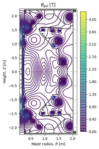
# total poloidal magnetic field

fig1, ax1 = plt.subplots(1, 1, figsize=(4, 8), dpi=100)

ax1.grid(True, which='both')
eq.tokamak.plot(axis=ax1,show=False)
# ax1.plot(tokamak.limiter.R, tokamak.limiter.Z, color='k', linewidth=1.2, linestyle="--")
ax1.plot(tokamak.wall.R, tokamak.wall.Z, color='k', linewidth=1.2, linestyle="-")
im1 = ax1.contour(eq.R, eq.Z, eq.Bpol(eq.R, eq.Z), levels=200)
ax1.set_aspect('equal')
ax1.set_xlim(0.1, 2.15)
ax1.set_ylim(-2.25, 2.25)
ax1.set_title(r"$B_{pol}$ [T]")
ax1.set_xlabel(r'Major radius, $R$ [m]')
ax1.set_ylabel(r'Height, $Z$ [m]')
cbar = plt.colorbar(im1, ax=ax1, fraction=0.09)

plt.tight_layout()
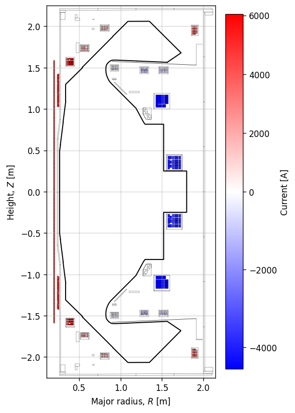
Coil currents
Here, we visualise the size of the currents in the poloidal field coils.
# listing the currents may not be that informative
eq.tokamak.getCurrents()
{'Solenoid': 5000.0,
 'PX': 4664.804998209495,
 'D1': 6037.479557316644,
 'D2': 1901.7767659342976,
 'D3': 1674.6060187513935,
 'Dp': -403.2350010512724,
 'D5': 3575.277366947996,
 'D6': -1090.53244932471,
 'D7': -568.10426314966,
 'P4': -4561.424627984298,
 'P5': -4036.498820520552,
 'P6': 0.0005657921621672163,
 'vessel_1': 0.0,
 'vessel_2': 0.0,
 'vessel_3': 0.0,
 'vessel_4': 0.0,
 'vessel_5': 0.0,
 'vessel_6': 0.0,
 'vessel_7': 0.0,
 'vessel_8': 0.0,
 'vessel_9': 0.0,
 'vessel_10': 0.0,
 'vessel_11': 0.0,
 'vessel_12': 0.0,
 'vessel_13': 0.0,
 'vessel_14': 0.0,
 'vessel_15': 0.0,
 'vessel_16': 0.0,
 'vessel_17': 0.0,
 'vessel_18': 0.0,
 'vessel_19': 0.0,
 'vessel_20': 0.0,
 'vessel_21': 0.0,
 'vessel_22': 0.0,
 'centrecolumn_1': 0.0,
 'centrecolumn_2': 0.0,
 'centrecolumn_3': 0.0,
 'centrecolumn_4': 0.0,
 'centrecolumn_5': 0.0,
 'centrecolumn_6': 0.0,
 'centrecolumn_7': 0.0,
 'centrecolumn_8': 0.0,
 'centrecolumn_9': 0.0,
 'centrecolumn_10': 0.0,
 'colosseum_upper_1': 0.0,
 'colosseum_upper_2': 0.0,
 'colosseum_upper_3': 0.0,
 'colosseum_lower_1': 0.0,
 'colosseum_lower_2': 0.0,
 'colosseum_lower_3': 0.0,
 'colosseum_outer_upper_1': 0.0,
 'colosseum_outer_upper_2': 0.0,
 'colosseum_outer_lower_1': 0.0,
 'colosseum_outer_lower_2': 0.0,
 'ring_plate_minor_upper_1': 0.0,
 'ring_plate_minor_upper_2': 0.0,
 'ring_plate_minor_lower_1': 0.0,
 'ring_plate_minor_lower_2': 0.0,
 'ring_plate_major_upper_1': 0.0,
 'ring_plate_major_lower_1': 0.0,
 'psp_upper_1': 0.0,
 'psp_lower_1': 0.0,
 'gas_baffle_upper_1': 0.0,
 'gas_baffle_upper_2': 0.0,
 'gas_baffle_upper_3': 0.0,
 'gas_baffle_lower_1': 0.0,
 'gas_baffle_lower_2': 0.0,
 'gas_baffle_lower_3': 0.0,
 'd1_case_upper_0': 0.0,
 'd1_case_upper_1': 0.0,
 'd1_case_upper_2': 0.0,
 'd1_case_upper_3': 0.0,
 'd1_case_lower_0': 0.0,
 'd1_case_lower_1': 0.0,
 'd1_case_lower_2': 0.0,
 'd1_case_lower_3': 0.0,
 'd2_case_upper_0': 0.0,
 'd2_case_upper_1': 0.0,
 'd2_case_upper_2': 0.0,
 'd2_case_upper_3': 0.0,
 'd2_case_lower_0': 0.0,
 'd2_case_lower_1': 0.0,
 'd2_case_lower_2': 0.0,
 'd2_case_lower_3': 0.0,
 'd3_case_upper_0': 0.0,
 'd3_case_upper_1': 0.0,
 'd3_case_upper_2': 0.0,
 'd3_case_upper_3': 0.0,
 'd3_case_lower_0': 0.0,
 'd3_case_lower_1': 0.0,
 'd3_case_lower_2': 0.0,
 'd3_case_lower_3': 0.0,
 'd5_case_upper_0': 0.0,
 'd5_case_upper_1': 0.0,
 'd5_case_upper_2': 0.0,
 'd5_case_upper_3': 0.0,
 'd5_case_lower_0': 0.0,
 'd5_case_lower_1': 0.0,
 'd5_case_lower_2': 0.0,
 'd5_case_lower_3': 0.0,
 'd6_case_upper_0': 0.0,
 'd6_case_upper_1': 0.0,
 'd6_case_upper_2': 0.0,
 'd6_case_upper_3': 0.0,
 'd6_case_lower_0': 0.0,
 'd6_case_lower_1': 0.0,
 'd6_case_lower_2': 0.0,
 'd6_case_lower_3': 0.0,
 'd7_case_upper_0': 0.0,
 'd7_case_upper_1': 0.0,
 'd7_case_upper_2': 0.0,
 'd7_case_upper_3': 0.0,
 'd7_case_lower_0': 0.0,
 'd7_case_lower_1': 0.0,
 'd7_case_lower_2': 0.0,
 'd7_case_lower_3': 0.0,
 'dp_case_upper_0': 0.0,
 'dp_case_upper_1': 0.0,
 'dp_case_upper_2': 0.0,
 'dp_case_upper_3': 0.0,
 'dp_case_lower_0': 0.0,
 'dp_case_lower_1': 0.0,
 'dp_case_lower_2': 0.0,
 'dp_case_lower_3': 0.0,
 'p4_case_upper_0': 0.0,
 'p4_case_upper_1': 0.0,
 'p4_case_upper_2': 0.0,
 'p4_case_upper_3': 0.0,
 'p4_case_lower_0': 0.0,
 'p4_case_lower_1': 0.0,
 'p4_case_lower_2': 0.0,
 'p4_case_lower_3': 0.0,
 'p5_case_upper_0': 0.0,
 'p5_case_upper_1': 0.0,
 'p5_case_upper_2': 0.0,
 'p5_case_upper_3': 0.0,
 'p5_case_lower_0': 0.0,
 'p5_case_lower_1': 0.0,
 'p5_case_lower_2': 0.0,
 'p5_case_lower_3': 0.0,
 'p6_case_upper_0': 0.0,
 'p6_case_upper_1': 0.0,
 'p6_case_upper_2': 0.0,
 'p6_case_upper_3': 0.0,
 'p6_case_upper_4': 0.0,
 'p6_case_lower_0': 0.0,
 'p6_case_lower_1': 0.0,
 'p6_case_lower_2': 0.0,
 'p6_case_lower_3': 0.0,
 'p6_case_lower_4': 0.0}
You can play around with the colour schemes below to visualise how the current is distributed around the machine. Note here that there is no current in the passive structures but they can be included if present.
from matplotlib.patches import Rectangle, Polygon
from matplotlib.colors import Normalize, TwoSlopeNorm
import matplotlib.cm as cm


# create colormap based on magnitude of currents
currents_array = []
for key in list(eq.tokamak.coils_dict.keys()):
    currents_array.append(eq.tokamak[key].current)

max_curr = np.max(np.abs(currents_array))
# norm = Normalize(vmin=-max_curr, vmax=max_curr) # alternative colorbar
norm = TwoSlopeNorm(vmin=np.min(currents_array), vcenter=0, vmax=np.max(currents_array))
cmap = cm.bwr


# plot
fig1, ax1 = plt.subplots(1, 1, figsize=(4, 8), dpi=120)
plt.tight_layout()
ax1.plot(tokamak.wall.R, tokamak.wall.Z, color='k', linewidth=1.2, linestyle="-")
ax1.grid(alpha=0.5)
ax1.set_aspect('equal')
ax1.set_xlim(0.1, 2.15)
ax1.set_ylim(-2.25, 2.25)
ax1.set_xlabel(r'Major radius, $R$ [m]')
ax1.set_ylabel(r'Height, $Z$ [m]')


for name in list(eq.tokamak.coils_dict.keys()):
    coil = eq.tokamak.coils_dict[name]
    current = eq.tokamak[name].current
    color = cmap(norm(current))  # map the current to a color

    # plot active coils (and currents)
    if coil["active"]:

        for i in range(0, len(coil["coords"][0,:])):
            patch = Rectangle(
                (coil["coords"][0,i] - coil["dR"] / 2, coil["coords"][1,i] - coil["dZ"] / 2),
                width=coil["dR"],
                height=coil["dZ"],
                facecolor=color,
                edgecolor='k',
                linewidth=0.2,
                )
            ax1.add_patch(patch)

    # plot passive structures (currents are zero here)
    else:
        patch = Polygon(
            coil["vertices"].T,
            facecolor=color,
            edgecolor="k",
            linewidth=0.2
        )
        ax1.add_patch(patch)


# add a colorbar
sm = cm.ScalarMappable(cmap=cmap, norm=norm)
sm.set_array([])
cbar = fig1.colorbar(sm, ax=ax1, orientation='vertical', fraction=0.09)
cbar.set_label('Current [A]')
Forces on the coils
We can also extract the radial and vertical forces on the coils.
eq.printForces()
Forces on coils
Solenoid (circuit)
  Solenoid : R = 7973.10 kN , Z = -0.00 kN
PX (circuit)
  PX1 : R = 222.67 kN , Z = 12.33 kN
  PX2 : R = 222.67 kN , Z = -12.33 kN
D1 (circuit)
  D11 : R = 322.25 kN , Z = -53.06 kN
  D12 : R = 322.25 kN , Z = 53.06 kN
D2 (circuit)
  D21 : R = 9.89 kN , Z = -15.13 kN
  D22 : R = 9.89 kN , Z = 15.13 kN
D3 (circuit)
  D31 : R = 9.51 kN , Z = -5.04 kN
  D32 : R = 9.51 kN , Z = 5.04 kN
Dp (circuit)
  Dp1 : R = 3.92 kN , Z = -1.05 kN
  Dp2 : R = 3.92 kN , Z = 1.05 kN
D5 (circuit)
  D51 : R = 52.21 kN , Z = -2.81 kN
  D52 : R = 52.21 kN , Z = 2.81 kN
D6 (circuit)
  D61 : R = 11.91 kN , Z = -11.33 kN
  D62 : R = 11.91 kN , Z = 11.33 kN
D7 (circuit)
  D71 : R = -0.94 kN , Z = -9.32 kN
  D72 : R = -0.94 kN , Z = 9.32 kN
P4 (circuit)
  P41 : R = 87.17 kN , Z = 14.26 kN
  P42 : R = 87.17 kN , Z = -14.26 kN
P5 (circuit)
  P51 : R = 114.57 kN , Z = 16.45 kN
  P52 : R = 114.57 kN , Z = -16.45 kN
P6 (circuit)
  P61 : R = -0.00 kN , Z = -0.00 kN
  P62 : R = 0.00 kN , Z = -0.00 kN
vessel_1 : R = 0.00 kN , Z = -0.00 kN
vessel_2 : R = 0.00 kN , Z = -0.00 kN
vessel_3 : R = 0.00 kN , Z = -0.00 kN
vessel_4 : R = 0.00 kN , Z = 0.00 kN
vessel_5 : R = 0.00 kN , Z = -0.00 kN
vessel_6 : R = 0.00 kN , Z = 0.00 kN
vessel_7 : R = 0.00 kN , Z = 0.00 kN
vessel_8 : R = 0.00 kN , Z = 0.00 kN
vessel_9 : R = 0.00 kN , Z = 0.00 kN
vessel_10 : R = 0.00 kN , Z = -0.00 kN
vessel_11 : R = 0.00 kN , Z = -0.00 kN
vessel_12 : R = 0.00 kN , Z = -0.00 kN
vessel_13 : R = 0.00 kN , Z = -0.00 kN
vessel_14 : R = 0.00 kN , Z = -0.00 kN
vessel_15 : R = 0.00 kN , Z = -0.00 kN
vessel_16 : R = 0.00 kN , Z = -0.00 kN
vessel_17 : R = 0.00 kN , Z = 0.00 kN
vessel_18 : R = 0.00 kN , Z = 0.00 kN
vessel_19 : R = 0.00 kN , Z = 0.00 kN
vessel_20 : R = 0.00 kN , Z = 0.00 kN
vessel_21 : R = 0.00 kN , Z = 0.00 kN
vessel_22 : R = 0.00 kN , Z = 0.00 kN
centrecolumn_1 : R = 0.00 kN , Z = 0.00 kN
centrecolumn_2 : R = 0.00 kN , Z = -0.00 kN
centrecolumn_3 : R = 0.00 kN , Z = -0.00 kN
centrecolumn_4 : R = 0.00 kN , Z = 0.00 kN
centrecolumn_5 : R = 0.00 kN , Z = 0.00 kN
centrecolumn_6 : R = 0.00 kN , Z = -0.00 kN
centrecolumn_7 : R = 0.00 kN , Z = 0.00 kN
centrecolumn_8 : R = 0.00 kN , Z = -0.00 kN
centrecolumn_9 : R = 0.00 kN , Z = 0.00 kN
centrecolumn_10 : R = 0.00 kN , Z = -0.00 kN
colosseum_upper_1 : R = 0.00 kN , Z = -0.00 kN
colosseum_upper_2 : R = 0.00 kN , Z = -0.00 kN
colosseum_upper_3 : R = 0.00 kN , Z = -0.00 kN
colosseum_lower_1 : R = 0.00 kN , Z = 0.00 kN
colosseum_lower_2 : R = 0.00 kN , Z = 0.00 kN
colosseum_lower_3 : R = 0.00 kN , Z = 0.00 kN
colosseum_outer_upper_1 : R = 0.00 kN , Z = -0.00 kN
colosseum_outer_upper_2 : R = 0.00 kN , Z = -0.00 kN
colosseum_outer_lower_1 : R = 0.00 kN , Z = 0.00 kN
colosseum_outer_lower_2 : R = 0.00 kN , Z = 0.00 kN
ring_plate_minor_upper_1 : R = 0.00 kN , Z = -0.00 kN
ring_plate_minor_upper_2 : R = 0.00 kN , Z = -0.00 kN
ring_plate_minor_lower_1 : R = 0.00 kN , Z = 0.00 kN
ring_plate_minor_lower_2 : R = 0.00 kN , Z = 0.00 kN
ring_plate_major_upper_1 : R = 0.00 kN , Z = -0.00 kN
ring_plate_major_lower_1 : R = 0.00 kN , Z = 0.00 kN
psp_upper_1 : R = 0.00 kN , Z = -0.00 kN
psp_lower_1 : R = 0.00 kN , Z = 0.00 kN
gas_baffle_upper_1 : R = 0.00 kN , Z = 0.00 kN
gas_baffle_upper_2 : R = 0.00 kN , Z = 0.00 kN
gas_baffle_upper_3 : R = 0.00 kN , Z = 0.00 kN
gas_baffle_lower_1 : R = 0.00 kN , Z = -0.00 kN
gas_baffle_lower_2 : R = 0.00 kN , Z = -0.00 kN
gas_baffle_lower_3 : R = 0.00 kN , Z = -0.00 kN
d1_case_upper_0 : R = 0.00 kN , Z = -0.00 kN
d1_case_upper_1 : R = 0.00 kN , Z = 0.00 kN
d1_case_upper_2 : R = 0.00 kN , Z = -0.00 kN
d1_case_upper_3 : R = 0.00 kN , Z = -0.00 kN
d1_case_lower_0 : R = 0.00 kN , Z = 0.00 kN
d1_case_lower_1 : R = 0.00 kN , Z = 0.00 kN
d1_case_lower_2 : R = 0.00 kN , Z = -0.00 kN
d1_case_lower_3 : R = 0.00 kN , Z = 0.00 kN
d2_case_upper_0 : R = 0.00 kN , Z = -0.00 kN
d2_case_upper_1 : R = 0.00 kN , Z = 0.00 kN
d2_case_upper_2 : R = 0.00 kN , Z = -0.00 kN
d2_case_upper_3 : R = 0.00 kN , Z = -0.00 kN
d2_case_lower_0 : R = 0.00 kN , Z = 0.00 kN
d2_case_lower_1 : R = 0.00 kN , Z = 0.00 kN
d2_case_lower_2 : R = 0.00 kN , Z = -0.00 kN
d2_case_lower_3 : R = 0.00 kN , Z = 0.00 kN
d3_case_upper_0 : R = 0.00 kN , Z = -0.00 kN
d3_case_upper_1 : R = 0.00 kN , Z = 0.00 kN
d3_case_upper_2 : R = 0.00 kN , Z = -0.00 kN
d3_case_upper_3 : R = 0.00 kN , Z = -0.00 kN
d3_case_lower_0 : R = 0.00 kN , Z = 0.00 kN
d3_case_lower_1 : R = 0.00 kN , Z = 0.00 kN
d3_case_lower_2 : R = 0.00 kN , Z = -0.00 kN
d3_case_lower_3 : R = 0.00 kN , Z = 0.00 kN
d5_case_upper_0 : R = 0.00 kN , Z = 0.00 kN
d5_case_upper_1 : R = 0.00 kN , Z = 0.00 kN
d5_case_upper_2 : R = 0.00 kN , Z = -0.00 kN
d5_case_upper_3 : R = 0.00 kN , Z = 0.00 kN
d5_case_lower_0 : R = 0.00 kN , Z = -0.00 kN
d5_case_lower_1 : R = 0.00 kN , Z = 0.00 kN
d5_case_lower_2 : R = 0.00 kN , Z = -0.00 kN
d5_case_lower_3 : R = 0.00 kN , Z = -0.00 kN
d6_case_upper_0 : R = 0.00 kN , Z = 0.00 kN
d6_case_upper_1 : R = 0.00 kN , Z = 0.00 kN
d6_case_upper_2 : R = 0.00 kN , Z = -0.00 kN
d6_case_upper_3 : R = 0.00 kN , Z = 0.00 kN
d6_case_lower_0 : R = 0.00 kN , Z = -0.00 kN
d6_case_lower_1 : R = 0.00 kN , Z = -0.00 kN
d6_case_lower_2 : R = 0.00 kN , Z = 0.00 kN
d6_case_lower_3 : R = 0.00 kN , Z = -0.00 kN
d7_case_upper_0 : R = 0.00 kN , Z = 0.00 kN
d7_case_upper_1 : R = 0.00 kN , Z = 0.00 kN
d7_case_upper_2 : R = 0.00 kN , Z = 0.00 kN
d7_case_upper_3 : R = 0.00 kN , Z = 0.00 kN
d7_case_lower_0 : R = 0.00 kN , Z = -0.00 kN
d7_case_lower_1 : R = 0.00 kN , Z = -0.00 kN
d7_case_lower_2 : R = 0.00 kN , Z = -0.00 kN
d7_case_lower_3 : R = 0.00 kN , Z = -0.00 kN
dp_case_upper_0 : R = 0.00 kN , Z = 0.00 kN
dp_case_upper_1 : R = 0.00 kN , Z = 0.00 kN
dp_case_upper_2 : R = 0.00 kN , Z = -0.00 kN
dp_case_upper_3 : R = 0.00 kN , Z = 0.00 kN
dp_case_lower_0 : R = 0.00 kN , Z = -0.00 kN
dp_case_lower_1 : R = 0.00 kN , Z = -0.00 kN
dp_case_lower_2 : R = 0.00 kN , Z = 0.00 kN
dp_case_lower_3 : R = 0.00 kN , Z = -0.00 kN
p4_case_upper_0 : R = 0.00 kN , Z = -0.00 kN
p4_case_upper_1 : R = 0.00 kN , Z = 0.00 kN
p4_case_upper_2 : R = 0.00 kN , Z = -0.00 kN
p4_case_upper_3 : R = 0.00 kN , Z = -0.00 kN
p4_case_lower_0 : R = 0.00 kN , Z = -0.00 kN
p4_case_lower_1 : R = 0.00 kN , Z = -0.00 kN
p4_case_lower_2 : R = 0.00 kN , Z = 0.00 kN
p4_case_lower_3 : R = 0.00 kN , Z = -0.00 kN
p5_case_upper_0 : R = 0.00 kN , Z = -0.00 kN
p5_case_upper_1 : R = 0.00 kN , Z = 0.00 kN
p5_case_upper_2 : R = 0.00 kN , Z = -0.00 kN
p5_case_upper_3 : R = 0.00 kN , Z = -0.00 kN
p5_case_lower_0 : R = 0.00 kN , Z = -0.00 kN
p5_case_lower_1 : R = 0.00 kN , Z = 0.00 kN
p5_case_lower_2 : R = 0.00 kN , Z = -0.00 kN
p5_case_lower_3 : R = 0.00 kN , Z = 0.00 kN
p6_case_upper_0 : R = 0.00 kN , Z = -0.00 kN
p6_case_upper_1 : R = 0.00 kN , Z = -0.00 kN
p6_case_upper_2 : R = 0.00 kN , Z = -0.00 kN
p6_case_upper_3 : R = 0.00 kN , Z = -0.00 kN
p6_case_upper_4 : R = 0.00 kN , Z = -0.00 kN
p6_case_lower_0 : R = 0.00 kN , Z = 0.00 kN
p6_case_lower_1 : R = 0.00 kN , Z = 0.00 kN
p6_case_lower_2 : R = 0.00 kN , Z = 0.00 kN
p6_case_lower_3 : R = 0.00 kN , Z = 0.00 kN
p6_case_lower_4 : R = 0.00 kN , Z = 0.00 kN
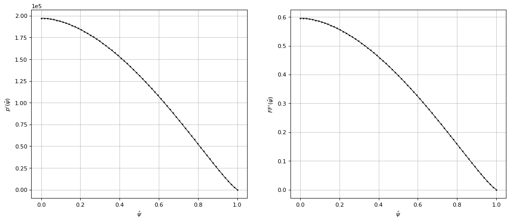
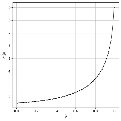
1D plasma current density profiles (and others)
Here, we visualise the \(p'\) and \(FF'\) profiles used in our equilbirium solve.
# plot the input p' and FF' profiles

psi_n = eq.psiN_1D(N=65)

fig1, (ax1, ax2) = plt.subplots(1, 2, figsize=(15,6), dpi=80)
ax1.grid(zorder=0, alpha=0.75)
ax1.plot(psi_n, profiles.pprime(psi_n), color='k', linewidth=1, marker='x', markersize=2, zorder=10)
ax1.set_xlabel(r'$\hat{\psi}$')
ax1.set_ylabel(r"$p'(\hat{\psi})$")
ax1.ticklabel_format(axis='y', scilimits=(0,0))

ax2.grid(zorder=0, alpha=0.75)
ax2.plot(psi_n, profiles.ffprime(psi_n), color='k', linewidth=1, marker='x', markersize=2, zorder=10)
ax2.set_xlabel(r'$\hat{\psi}$')
ax2.set_ylabel(r"$FF'(\hat{\psi})$")
Text(0, 0.5, "$FF'(\\hat{\\psi})$")
# plot q profile

psi_n = np.linspace(0.01,0.99,65)  # values of q at 0 and 1 can be problematic

fig1, ax1 = plt.subplots(1, 1, figsize=(6,6), dpi=80)
ax1.grid(zorder=0, alpha=0.75)
ax1.plot(psi_n, eq.q(psi_n), color='k', linewidth=1, marker='x', markersize=2, zorder=10)
ax1.set_xlabel(r'$\hat{\psi}$')
ax1.set_ylabel(r"$q(\hat{\psi})$")
Text(0, 0.5, '$q(\\hat{\\psi})$')
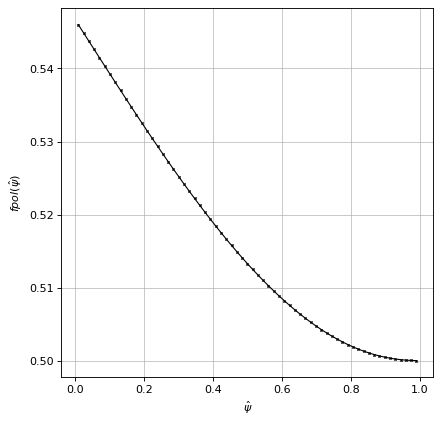
# plot fpol

fig1, ax1 = plt.subplots(1, 1, figsize=(6,6), dpi=80)
ax1.grid(zorder=0, alpha=0.75)
ax1.plot(psi_n, eq.fpol(psi_n), color='k', linewidth=1, marker='x', markersize=2, zorder=10)
ax1.set_xlabel(r'$\hat{\psi}$')
ax1.set_ylabel(r"$fpol(\hat{\psi})$")
Text(0, 0.5, '$fpol(\\hat{\\psi})$')
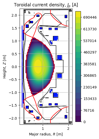
Toroidal current density
Here, we visualise the toroidal current density inside the core of the plasma.
fig1, ax1 = plt.subplots(1, 1, figsize=(4, 8), dpi=100)

ax1.grid(True, which='both')
eq.tokamak.plot(axis=ax1,show=False)
ax1.plot(tokamak.wall.R, tokamak.wall.Z, color='k', linewidth=1.2, linestyle="-")
im1 = ax1.contourf(eq.R, eq.Z, eq._profiles.jtor, levels=np.linspace(0.01, np.max( eq._profiles.jtor,), 20))
ax1.contour(eq.R, eq.Z, eq.psi(), levels=[eq.psi_bndry], colors='r')
ax1.set_aspect('equal')
ax1.set_xlim(0.1, 2.15)
ax1.set_ylim(-2.25, 2.25)
ax1.set_title(r"Toroidal current density, $J_p$ [A]")
ax1.set_xlabel(r'Major radius, $R$ [m]')
ax1.set_ylabel(r'Height, $Z$ [m]')
cbar = plt.colorbar(im1, ax=ax1, fraction=0.09)

plt.tight_layout()
# # plot 1D_jtor
# fig1, ax1 = plt.subplots(1, 1, figsize=(6,6), dpi=80)
# ax1.grid(zorder=0, alpha=0.75)
# ax1.plot(eq.psiN_1D(N=101), eq.jtor_1D(N=101), color='k', linewidth=1, marker='x', markersize=2, zorder=10)
# ax1.set_xlabel(r'$\hat{\psi}$')
# ax1.set_ylabel(r"$J_{tor}(\hat{\psi})$")
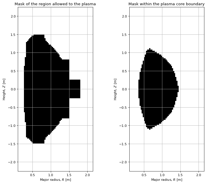
Masking arrays
There are a number of masking arrays that are built during the equilibrium solve that may be useful for plotting or other calculations you may carry out.
fig1, (ax1, ax2) = plt.subplots(1, 2, figsize=(10, 8), dpi=80)
plt.subplots_adjust(wspace=0.25)  # adjust the horizontal space between subplots

ax1.grid(True, which='both')
# eq.tokamak.plot(axis=ax1,show=False)
# ax1.fill(tokamak.wall.R, tokamak.wall.Z, color='k', linewidth=1.2, facecolor=None, zorder=0)
# ax1.contour(eq.R, eq.Z, eq.psi(), levels=[eq.psi_bndry], linestyles='solid', colors='r') #, label="Separatrix")
ax1.pcolormesh(eq.R, eq.Z, eq.mask_inside_limiter, cmap="Greys")
ax1.set_aspect('equal')
ax1.set_xlim(0.1, 2.15)
ax1.set_ylim(-2.25, 2.25)
ax1.set_xlabel(r'Major radius, $R$ [m]')
ax1.set_ylabel(r'Height, $Z$ [m]')
ax1.set_title("Mask of the region allowed to the plasma")


ax2.grid(True, which='both')
# eq.tokamak.plot(axis=ax2,show=False)
# ax2.fill(tokamak.wall.R, tokamak.wall.Z, color='k', linewidth=1.2, facecolor=None, zorder=0)
# ax2.contour(eq.R, eq.Z, eq.psi(), levels=[eq.psi_bndry], linestyles='solid', colors='r') #, label="Separatrix")
ax2.pcolormesh(eq.R, eq.Z, eq._profiles.diverted_core_mask, cmap="Greys")
ax2.set_aspect('equal')
ax2.set_xlim(0.1, 2.15)
ax2.set_ylim(-2.25, 2.25)
ax2.set_xlabel(r'Major radius, $R$ [m]')
ax2.set_ylabel(r'Height, $Z$ [m]')
ax2.set_title("Mask within the plasma core boundary")

plt.tight_layout()