Example: Static inverse free-boundary equilibrium calculations (in SPARC)

---

Here we will generate an equilibrium (find coil currents with the inverse solver) in a SPARC-like tokamak.

The machine description comes from files located here.

The equilbirium\profile parameters are completely made up - please experiment on your own and change them to more realistic values as you please!

Import packages

import matplotlib.pyplot as plt
import numpy as np

Create the machine object

# build machine
from freegsnke import build_machine
tokamak = build_machine.tokamak(
    active_coils_path=f"../machine_configs/SPARC/SPARC_active_coils.pickle",
    passive_coils_path=f"../machine_configs/SPARC/SPARC_passive_coils.pickle",
    limiter_path=f"../machine_configs/SPARC/SPARC_limiter.pickle",
    wall_path=f"../machine_configs/SPARC/SPARC_wall.pickle",
)

Active coils --> built from pickle file.
Passive structures --> built from pickle file.
Limiter --> built from pickle file.
Wall --> built from pickle file.

Magnetic probes --> none provided.

Resistance (R) and inductance (M) matrices --> built using actives (and passives if present).
Tokamak built.

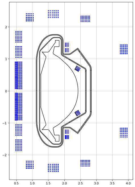
fig1, ax1 = plt.subplots(1, 1, figsize=(7, 15), dpi=80)

ax1.grid(zorder=0, alpha=0.75)
ax1.set_aspect('equal')
tokamak.plot(axis=ax1,show=False)                                                          # plots the active coils and passive structures
ax1.fill(tokamak.wall.R, tokamak.wall.Z, color='k', linewidth=1.2, facecolor='w', zorder=0)   # plots the limiter

[<matplotlib.patches.Polygon at 0x1528a50c0>]

Instantiate an equilibrium

from freegsnke import equilibrium_update

eq = equilibrium_update.Equilibrium(
    tokamak=tokamak,      # provide tokamak object
    Rmin=1.1, Rmax=2.7,   # radial range
    Zmin=-1.8, Zmax=1.8,  # vertical range
    nx=129,                # number of grid points in the radial direction (needs to be of the form (2**n + 1) with n being an integer)
    ny=129,                # number of grid points in the vertical direction (needs to be of the form (2**n + 1) with n being an integer)
    # psi=plasma_psi
)

Instantiate a profile object

# initialise the profiles
from freegsnke.jtor_update import ConstrainPaxisIp
profiles = ConstrainPaxisIp(
    eq=eq,        # equilibrium object
    paxis=5e4,    # pressure on axis
    Ip=8.7e6,       # plasma current
    fvac=0.5,     # fvac = rB_{tor}
    alpha_m=1.8,  # profile function parameter
    alpha_n=1.2   # profile function parameter
)

Load the static nonlinear solver

from freegsnke import GSstaticsolver
GSStaticSolver = GSstaticsolver.NKGSsolver(eq)    

Constraints

Rx = 1.55      # X-point radius
Zx = 1.15      # X-point height

# set desired null_points locations
# this can include X-point and O-point locations
null_points = [[Rx, Rx], [Zx, -Zx]]

Rout = 2.4    # outboard midplane radius
Rin = 1.3    # inboard midplane radius

# set desired isoflux constraints with format 
# isoflux_set = [isoflux_0, isoflux_1 ... ] 
# with each isoflux_i = [R_coords, Z_coords]
isoflux_set = np.array([[[Rx, Rx, Rout, Rin, 1.7, 1.7], [Zx, -Zx, 0.0, 0.0, 1.5, -1.5]]])
           
# instantiate the freegsnke constrain object
from freegsnke.inverse import Inverse_optimizer
constrain = Inverse_optimizer(null_points=null_points,
                              isoflux_set=isoflux_set)

The inverse solve

GSStaticSolver.inverse_solve(eq=eq, 
                     profiles=profiles, 
                     constrain=constrain, 
                     target_relative_tolerance=1e-6,
                     target_relative_psit_update=1e-3,
                     verbose=False, # print output
                     l2_reg=np.array([1e-16]*10 + [1e-5]), 
                     )
                     

Inverse static solve SUCCESS. Tolerance 3.65e-07 (vs. requested 1e-06) reached in 11/100 iterations.

# refine with a forward solve (now the currents are known)
GSStaticSolver.solve(eq=eq, 
                     profiles=profiles, 
                     constrain=None, 
                     target_relative_tolerance=1e-9,
                     verbose=False, # print output
                     )

Forward static solve SUCCESS. Tolerance 2.14e-10 (vs. requested 1.00e-09) reached in 4/100 iterations.

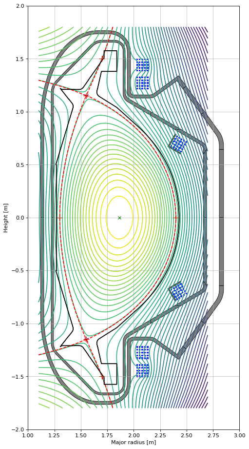
fig1, ax1 = plt.subplots(1, 1, figsize=(7, 15), dpi=80)

ax1.grid(zorder=0, alpha=0.75)
ax1.set_aspect('equal')
eq.tokamak.plot(axis=ax1,show=False)                                                          # plots the active coils and passive structures
ax1.fill(tokamak.wall.R, tokamak.wall.Z, color='k', linewidth=1.2, facecolor='w', zorder=0)   # plots the limiter
eq.plot(axis=ax1,show=False)                                                                  # plots the equilibrium
constrain.plot(axis=ax1, show=False)                                                          # plots the contraints
ax1.set_xlim(1.0, 3.0)
ax1.set_ylim(-2.0, 2.0)

(-2.0, 2.0)

eq.tokamak.getCurrents()

# # save coil currents to file
# import pickle
# with open('simple_diverted_currents_PaxisIp.pk', 'wb') as f:
#     pickle.dump(obj=inverse_current_values, file=f)

{'CS1I': -67750.4895278049,
 'CS1O': -61587.99877444454,
 'CS2': -162906.56986075832,
 'CS3': 58001.720719223755,
 'PF1': 100420.28963501936,
 'PF2': 88283.60063791212,
 'PF3': -97548.58916319988,
 'PF4': -140162.231729873,
 'DV1': 19990.499914512042,
 'DV2': -8231.20219673651,
 'VS1': 0.0057785679935671,
 'vacuum_vessel_0': 0.0,
 'vacuum_vessel_1': 0.0,
 'vacuum_vessel_2': 0.0,
 'vacuum_vessel_3': 0.0,
 'vacuum_vessel_4': 0.0,
 'vacuum_vessel_5': 0.0,
 'vacuum_vessel_6': 0.0,
 'vacuum_vessel_7': 0.0,
 'vacuum_vessel_8': 0.0,
 'vacuum_vessel_9': 0.0,
 'vacuum_vessel_10': 0.0,
 'vacuum_vessel_11': 0.0,
 'vacuum_vessel_12': 0.0,
 'vacuum_vessel_13': 0.0,
 'vacuum_vessel_14': 0.0,
 'vacuum_vessel_15': 0.0,
 'VSC_coil_cover0': 0.0,
 'VSC_coil_cover1': 0.0}