Example: Saving an equilibrium to geqdsk (via FreeQDSK)

In this example, we take a MAST-U-like equilibrium and show how to save it to geqdsk file via the FreeQDSK package.

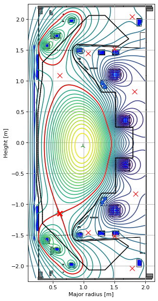
As in the previous example, we run our standard equilibrium solve - making it lower single null by pushing the P6 current.

import matplotlib.pyplot as plt
import numpy as np

# build machine
from freegsnke import build_machine
tokamak = build_machine.tokamak(
    active_coils_path=f"../machine_configs/MAST-U/MAST-U_like_active_coils.pickle",
    passive_coils_path=f"../machine_configs/MAST-U/MAST-U_like_passive_coils.pickle",
    limiter_path=f"../machine_configs/MAST-U/MAST-U_like_limiter.pickle",
    wall_path=f"../machine_configs/MAST-U/MAST-U_like_wall.pickle",
)

# initialise equilibrium object
from freegsnke import equilibrium_update
eq = equilibrium_update.Equilibrium(
    tokamak=tokamak,
    Rmin=0.1, Rmax=2.0,   # radial range
    Zmin=-2.2, Zmax=2.2,  # vertical range
    nx=65,                # number of grid points in the radial direction (needs to be of the form (2**n + 1) with n being an integer)
    ny=129,               # number of grid points in the vertical direction (needs to be of the form (2**n + 1) with n being an integer)
)  

# initialise profile object
from freegsnke.jtor_update import ConstrainPaxisIp
profiles = ConstrainPaxisIp(
    eq=eq,
    paxis=8.1e3,
    Ip=6.2e5,
    fvac=0.5,
    alpha_m=1.8,
    alpha_n=1.2
)

# initialise solver
from freegsnke import GSstaticsolver
GSStaticSolver = GSstaticsolver.NKGSsolver(eq)    

# set coil currents
import pickle
with open('data/simple_diverted_currents_PaxisIp.pk', 'rb') as f:
    current_values = pickle.load(f)

for key in current_values.keys():
    eq.tokamak[key].current = current_values[key]
    
# change this to shift plasma vertically up (-) or down (+)
eq.tokamak["P6"].current += 500

# carry out forward solve
GSStaticSolver.solve(eq=eq, 
                     profiles=profiles, 
                     constrain=None, 
                     target_relative_tolerance=1e-9)

# plot the resulting equilibrium
fig1, ax1 = plt.subplots(1, 1, figsize=(4, 8), dpi=80)
ax1.grid(True, which='both')
eq.plot(axis=ax1, show=False)
eq.tokamak.plot(axis=ax1, show=False)
ax1.set_xlim(0.1, 2.15)
ax1.set_ylim(-2.25, 2.25)
plt.tight_layout()

Active coils --> built from pickle file.
Passive structures --> built from pickle file.
Limiter --> built from pickle file.
Wall --> built from pickle file.

Magnetic probes --> none provided.

Resistance (R) and inductance (M) matrices --> built using actives (and passives if present).
Tokamak built.

Forward static solve SUCCESS. Tolerance 4.04e-10 (vs. requested 1.00e-09) reached in 26/100 iterations.

Writing a geqdsk file

FreeQDSK writes a geqdsk file via geqdsk.write(data, f), where data contains a dictionary of key equilbirium information (see below).

from freeqdsk import geqdsk

# grid quantities
nx, ny = eq.nx, eq.ny
R_1D, Z_1D = eq.R_1D, eq.Z_1D
rmin, rmax = R_1D[0], R_1D[-1]
zmin, zmax = Z_1D[0], Z_1D[-1]

# vacuum field
# fvac = R*Btor in vacuum (constant); rcentr is an arbitrary reference radius
# convention: often taken as the machine geometric centre or R at magnetic axis
rcentr = 0.5 * (rmin + rmax)          # assumed — check against your COCOS/convention
bcentr = profiles.fvac() / rcentr     # fvac passed into ConstrainPaxisIp as 0.5

# magnetic axis
rmagx, zmagx = eq.magneticAxis()[0:2]

# last closed flux surface (i.e. core plasma boundary)
sep = eq.separatrix(ntheta=180)        # (R, Z) points around LCFS
rbdry, zbdry = sep[:, 0], sep[:, 1]

# wall contour
rlim, zlim = eq.tokamak.wall.R, eq.tokamak.wall.Z

# 1D normalised psi
psi_n = eq.psiN_1D(N=nx)

# store all in dictionary (See FreeQDSK docs for details)
data = {
    "comment": "FreeGSNKE equilibrium",
    "shot": 0,
    "nx": nx,
    "ny": ny,
    "rdim": rmax - rmin,
    "zdim": zmax - zmin,
    "rcentr": rcentr,
    "bcentr": bcentr,
    "rleft": rmin,
    "zmid": 0.5 * (zmin + zmax),
    "rmagx": rmagx,
    "zmagx": zmagx,
    "simagx": eq.psi_axis,
    "sibdry": eq.psi_bndry,
    "cpasma": eq.plasmaCurrent(),
    "fpol": profiles.fpol(psi_n),
    "pres": profiles.pressure(psi_n),
    "ffprime": profiles.ffprime(psi_n),
    "pprime": profiles.pprime(psi_n),
    "psi": eq.psi(),
    "qpsi": eq.q(psi_n),
    "nbdry": len(rbdry),
    "rbdry": rbdry,
    "zbdry": zbdry,
    "nlim": len(rlim),
    "rlim": rlim,
    "zlim": zlim,
}

psinorm contains 0 or 1, which may cause numerical issues druing safety factor calculation.

# save the file!
with open("MASTU_LSN.geqdsk", "w") as f:
    geqdsk.write(data, f)

Reading a geqdsk file

FreeQDSK can also read a geqdsk file back in via geqdsk.read(f), returning the same kind of dictionary we just wrote.

A geqdsk file doesn’t store individual coil currents, so we need use the inverse solver to re-build the equilibrium, using the stored 2D psi map (and other data) as constraints.

We build the constraints entirely from what the geqdsk file gives us:

• an isoflux constraint from the last closed flux surface (rbdry/zbdry) - all these points should sit on the same flux contour, without us needing to know its absolute value;

• null-point constraints at the magnetic axis (rmagx/zmagx, also from the file);

• a psi_vals constraint built from the entire saved 2D psi map - unlike the constraints above, this one is given the actual flux values, not just which points should share a value, so it’s what lets the optimiser pin down the absolute flux level (and, with it, the individual coil currents) rather than just the plasma shape.

To check that the file faithfully captures the equilibrium, we’ll reconstruct it purely from what’s in the geqdsk file: the grid extent, the plasma current (cpasma), and the p'(ψ_n)/FF'(ψ_n) profile data (pprime/ffprime).

FreeGSNKE’s GeneralPprimeFFprime profile class accepts exactly this kind of tabulated profile data directly, rather than a parametric form like ConstrainPaxisIp above.

We reset the coil currents on a fresh, independent tokamak to zero first, to make sure we aren’t just reusing the answer.

# open the file!
with open("MASTU_LSN.geqdsk", "r") as f:
    freeqdsk_data = geqdsk.read(f)

from freegsnke.jtor_update import GeneralPprimeFFprime

# grid data
Rmin = freeqdsk_data["rleft"]
Rmax = Rmin + freeqdsk_data["rdim"]
Zmin = freeqdsk_data["zmid"] - 0.5 * freeqdsk_data["zdim"]
Zmax = freeqdsk_data["zmid"] + 0.5 * freeqdsk_data["zdim"]
nx_read, ny_read = freeqdsk_data["nx"], freeqdsk_data["ny"]

# normalised psi
psi_n_read = np.linspace(0, 1, nx_read)

Now let’s set up and run the inverse solver, using those quantities plus the constraints described above to reconstruct the coil currents.

from freegsnke.inverse import Inverse_optimizer

# coil names
active_coil_names = tokamak.coils_list[: tokamak.n_active_coils]

# fresh tokamak so we can set coil currents to zero and compare to old eq object
tokamak_inv = build_machine.tokamak(
    active_coils_path=f"../machine_configs/MAST-U/MAST-U_like_active_coils.pickle",
    passive_coils_path=f"../machine_configs/MAST-U/MAST-U_like_passive_coils.pickle",
    limiter_path=f"../machine_configs/MAST-U/MAST-U_like_limiter.pickle",
    wall_path=f"../machine_configs/MAST-U/MAST-U_like_wall.pickle",
)

# fresh equilibrium object
eq_inv = equilibrium_update.Equilibrium(
    tokamak=tokamak_inv,
    Rmin=Rmin, Rmax=Rmax,
    Zmin=Zmin, Zmax=Zmax,
    nx=nx_read,
    ny=ny_read,
)

# fresh profiles object
profiles_inv = GeneralPprimeFFprime(
    eq=eq_inv,
    Ip=freeqdsk_data["cpasma"],
    fvac=freeqdsk_data["bcentr"] * freeqdsk_data["rcentr"],
    psi_n=psi_n_read,
    pprime_data=freeqdsk_data["pprime"],
    ffprime_data=freeqdsk_data["ffprime"],
)

# isoflux constraint: subsample the LCFS boundary stored in the geqdsk file
isoflux_set = [[freeqdsk_data["rbdry"][::5], freeqdsk_data["zbdry"][::5]]]

# null-point constraints: magnetic axis (from the file)
null_points = [
    [freeqdsk_data["rmagx"]],
    [freeqdsk_data["zmagx"]],
]

# psi_vals constraint built from the *entire* saved 2D psi map. Passing the grid's own
# (R, Z) meshgrids (rather than a sparse list of points) triggers Inverse_optimizer's
# "full grid" fast path, which reuses the equilibrium's own cached Greens functions
# instead of recomputing them pointwise.
psi_vals = [eq_inv.R, eq_inv.Z, freeqdsk_data["psi"]]

# build constraints
constrain = Inverse_optimizer(
    isoflux_set=isoflux_set,
    null_points=null_points,
    psi_vals=psi_vals,
)

# initialise solver object
GSStaticSolver_inv = GSstaticsolver.NKGSsolver(eq_inv)

Active coils --> built from pickle file.
Passive structures --> built from pickle file.
Limiter --> built from pickle file.
Wall --> built from pickle file.

Magnetic probes --> none provided.

Resistance (R) and inductance (M) matrices --> built using actives (and passives if present).
Tokamak built.

# set coils to zero current
for label in active_coil_names:
    eq_inv.tokamak.set_coil_current(label, 0.0)

# default plasma flux guess
eq_inv.set_plasma_psi(eq_inv.create_psi_plasma_default())

# solve
GSStaticSolver_inv.solve(
    eq=eq_inv,
    profiles=profiles_inv,
    constrain=constrain,
    target_relative_tolerance=1e-4,
    target_relative_psit_update=1e-3,
    max_solving_iterations=50,
    l2_reg=1e-9,
    verbose=True,
    Picard_handover=1e-5,
    full_jacobian_handover=[2e-2,1e-2],
)

-----
Inverse static solve starting...

Successfully computed GS residual using initial plasma_psi and tokamak_psi guesses.
Initial relative error = 1.00e+00
-----
Iteration: 0
Using simplified Green's Jacobian (of constraints wrt coil currents) to optimise the currents.
Change in coil currents (being controlled): ['-2.03e+05', '2.95e+04', '-1.80e+04', '-2.68e+04', '-1.45e+04', '-9.09e+03', '6.89e+03', '-9.85e+03', '2.05e+03', '-4.74e+03', '-2.42e+03', '-5.55e+02']
Constraint losses = 5.69e+00
Relative update of tokamak psi (in plasma core): 4.04e+07
Handing off to forward solve (with updated currents).
Relative error =  9.50e-01
-----
Iteration: 1
Using simplified Green's Jacobian (of constraints wrt coil currents) to optimise the currents.
Change in coil currents (being controlled): ['6.35e+04', '-8.83e+03', '7.58e+03', '9.50e+03', '5.33e+03', '1.88e+03', '-2.01e+03', '2.84e+03', '-3.55e+02', '1.55e+02', '-6.10e+02', '9.40e+01']
Constraint losses = 3.31e+00
Relative update of tokamak psi (in plasma core): 1.79e-01
Handing off to forward solve (with updated currents).
Relative error =  8.66e-01
-----
Iteration: 2
Using simplified Green's Jacobian (of constraints wrt coil currents) to optimise the currents.
Change in coil currents (being controlled): ['4.72e+04', '-6.54e+03', '5.63e+03', '7.05e+03', '3.96e+03', '1.40e+03', '-1.49e+03', '2.12e+03', '-2.79e+02', '1.36e+02', '-4.07e+02', '8.59e+01']
Constraint losses = 2.31e+00
Relative update of tokamak psi (in plasma core): 1.80e-01
Handing off to forward solve (with updated currents).
Relative error =  7.55e-01
-----
Iteration: 3
Using simplified Green's Jacobian (of constraints wrt coil currents) to optimise the currents.
Change in coil currents (being controlled): ['3.51e+04', '-4.87e+03', '4.18e+03', '5.23e+03', '2.94e+03', '1.04e+03', '-1.11e+03', '1.58e+03', '-2.25e+02', '1.22e+02', '-2.46e+02', '7.87e+01']
Constraint losses = 1.58e+00
Relative update of tokamak psi (in plasma core): 1.78e-01
Handing off to forward solve (with updated currents).
Relative error =  6.11e-01
-----
Iteration: 4
Using simplified Green's Jacobian (of constraints wrt coil currents) to optimise the currents.
Change in coil currents (being controlled): ['2.60e+04', '-3.68e+03', '3.10e+03', '3.88e+03', '2.18e+03', '7.76e+02', '-8.25e+02', '1.19e+03', '-1.89e+02', '1.13e+02', '-1.06e+02', '7.31e+01']
Constraint losses = 1.07e+00
Relative update of tokamak psi (in plasma core): 1.73e-01
Handing off to forward solve (with updated currents).
Relative error =  4.25e-01
-----
Iteration: 5
Using simplified Green's Jacobian (of constraints wrt coil currents) to optimise the currents.
Change in coil currents (being controlled): ['1.88e+04', '-2.34e+03', '2.25e+03', '2.81e+03', '1.57e+03', '6.04e+02', '-6.03e+02', '8.75e+02', '-1.63e+02', '1.35e+02', '-4.90e+01', '7.94e+01']
Constraint losses = 7.52e-01
Relative update of tokamak psi (in plasma core): 1.79e-01
Handing off to forward solve (with updated currents).
Relative error =  1.73e-01
-----
Iteration: 6
Using simplified Green's Jacobian (of constraints wrt coil currents) to optimise the currents.
Change in coil currents (being controlled): ['7.63e+03', '7.22e+02', '8.44e+02', '1.03e+03', '4.31e+02', '8.29e+02', '-5.44e+02', '5.70e+02', '-1.65e+02', '2.10e+02', '1.62e+01', '1.03e+02']
Constraint losses = 5.99e-01
Relative update of tokamak psi (in plasma core): 1.15e-01
Handing off to forward solve (with updated currents).
Relative error =  9.56e-03
-----
Iteration: 7
Using simplified Green's Jacobian (of constraints wrt coil currents) to optimise the currents.
Change in coil currents (being controlled): ['5.61e+03', '6.32e+02', '7.32e+02', '8.93e+02', '4.96e+02', '3.44e+02', '-1.46e+02', '2.77e+02', '-1.42e+02', '2.95e+02', '-2.09e+02', '4.31e+01']
Constraint losses = 5.65e-01
Relative update of tokamak psi (in plasma core): 9.48e-02
Handing off to forward solve (with updated currents).
Relative error =  1.10e-02
-----
Iteration: 8
Using simplified Green's Jacobian (of constraints wrt coil currents) to optimise the currents.
Change in coil currents (being controlled): ['2.15e+03', '-3.61e+01', '2.70e+02', '4.38e+02', '3.10e+02', '-1.39e+02', '4.42e+01', '3.91e+01', '-5.95e+00', '3.31e+00', '3.55e+01', '7.95e+01']
Constraint losses = 5.42e-01
Relative update of tokamak psi (in plasma core): 4.13e-02
Handing off to forward solve (with updated currents).
Relative error =  7.87e-03
-----
Iteration: 9
Using simplified Green's Jacobian (of constraints wrt coil currents) to optimise the currents.
Change in coil currents (being controlled): ['9.44e+02', '-1.96e+02', '1.08e+02', '2.05e+02', '1.29e+02', '-8.52e+01', '2.06e+01', '1.71e+01', '2.17e+00', '-5.39e+00', '-2.35e+00', '5.53e+00']
Constraint losses = 5.40e-01
Relative update of tokamak psi (in plasma core): 1.70e-02
Handing off to forward solve (with updated currents).
Relative error =  8.46e-03
-----
Iteration: 10
Using simplified Green's Jacobian (of constraints wrt coil currents) to optimise the currents.
Change in coil currents (being controlled): ['4.38e+02', '-1.89e+02', '6.00e+01', '9.75e+01', '5.33e+01', '-3.77e+01', '9.13e+00', '8.23e+00', '9.71e-01', '-2.48e+00', '-2.50e+00', '3.88e-02']
Constraint losses = 5.39e-01
Relative update of tokamak psi (in plasma core): 7.62e-03
Handing off to forward solve (with updated currents).
Relative error =  9.16e-03
-----
Iteration: 11
Using full Jacobian (of constraints wrt coil currents) to optimsise currents.

 - calculating derivatives for coil 1/12
 - calculating derivatives for coil 2/12
 - calculating derivatives for coil 3/12
 - calculating derivatives for coil 4/12
 - calculating derivatives for coil 5/12
 - calculating derivatives for coil 6/12
 - calculating derivatives for coil 7/12
 - calculating derivatives for coil 8/12
 - calculating derivatives for coil 9/12

 - calculating derivatives for coil 10/12
 - calculating derivatives for coil 11/12
 - calculating derivatives for coil 12/12
Change in coil currents (being controlled): ['4.29e+01', '7.51e+01', '8.74e+01', '4.36e+01', '5.32e+00', '-7.39e+01', '-1.31e+01', '2.74e+01', '-9.93e+00', '-2.19e+00', '9.48e+01', '3.46e+02']
Constraint losses = 1.71e+00
Relative update of tokamak psi (in plasma core): 8.16e-03
Handing off to forward solve (with updated currents).
Relative error =  1.45e-02
-----
Iteration: 12
Using full Jacobian (of constraints wrt coil currents) to optimsise currents.

 - calculating derivatives for coil 1/12
 - calculating derivatives for coil 2/12
 - calculating derivatives for coil 3/12
 - calculating derivatives for coil 4/12
 - calculating derivatives for coil 5/12
 - calculating derivatives for coil 6/12
 - calculating derivatives for coil 7/12

 - calculating derivatives for coil 8/12
 - calculating derivatives for coil 9/12
 - calculating derivatives for coil 10/12
 - calculating derivatives for coil 11/12
 - calculating derivatives for coil 12/12
Change in coil currents (being controlled): ['5.26e+01', '-3.57e+01', '-2.45e+01', '-5.12e+00', '1.01e+00', '1.88e+01', '9.99e+00', '-1.18e-01', '2.34e+00', '1.09e+01', '-6.16e+01', '5.56e+01']
Constraint losses = 1.71e+00
Relative update of tokamak psi (in plasma core): 3.28e-03
Handing off to forward solve (with updated currents).
Relative error =  2.76e-03
-----
Iteration: 13
Using full Jacobian (of constraints wrt coil currents) to optimsise currents.

 - calculating derivatives for coil 1/12
 - calculating derivatives for coil 2/12
 - calculating derivatives for coil 3/12
 - calculating derivatives for coil 4/12
 - calculating derivatives for coil 5/12
 - calculating derivatives for coil 6/12
 - calculating derivatives for coil 7/12

 - calculating derivatives for coil 8/12
 - calculating derivatives for coil 9/12
 - calculating derivatives for coil 10/12
 - calculating derivatives for coil 11/12
 - calculating derivatives for coil 12/12
Change in coil currents (being controlled): ['3.94e+01', '-3.43e+01', '-1.60e+01', '-1.30e+00', '5.44e+00', '9.76e+00', '3.49e+00', '-1.32e+00', '-4.68e+00', '6.99e+00', '-4.99e+00', '1.47e+01']
Constraint losses = 1.71e+00
Relative update of tokamak psi (in plasma core): 5.73e-04
Handing off to forward solve (with updated currents).
Relative error =  6.09e-04
-----
Iteration: 14
Using full Jacobian (of constraints wrt coil currents) to optimsise currents.
 - calculating derivatives for coil 1/12

 - calculating derivatives for coil 2/12
 - calculating derivatives for coil 3/12
 - calculating derivatives for coil 4/12
 - calculating derivatives for coil 5/12
 - calculating derivatives for coil 6/12
 - calculating derivatives for coil 7/12
 - calculating derivatives for coil 8/12
 - calculating derivatives for coil 9/12

 - calculating derivatives for coil 10/12
 - calculating derivatives for coil 11/12
 - calculating derivatives for coil 12/12
Change in coil currents (being controlled): ['3.18e+01', '-2.79e+01', '-7.60e+00', '2.62e+00', '5.88e+00', '8.62e+00', '-8.58e-01', '-1.07e+01', '3.30e+00', '9.30e+00', '1.46e+00', '4.20e+00']
Constraint losses = 1.71e+00
Relative update of tokamak psi (in plasma core): 8.65e-04
Handing off to forward solve (with updated currents).
Relative error =  2.37e-04
-----
Iteration: 15
Using full Jacobian (of constraints wrt coil currents) to optimsise currents.

 - calculating derivatives for coil 1/12
 - calculating derivatives for coil 2/12
 - calculating derivatives for coil 3/12
 - calculating derivatives for coil 4/12
 - calculating derivatives for coil 5/12
 - calculating derivatives for coil 6/12
 - calculating derivatives for coil 7/12

 - calculating derivatives for coil 8/12
 - calculating derivatives for coil 9/12
 - calculating derivatives for coil 10/12
 - calculating derivatives for coil 11/12
 - calculating derivatives for coil 12/12
Change in coil currents (being controlled): ['2.91e+01', '-2.62e+01', '-5.56e+00', '1.60e+00', '1.90e+00', '1.11e+00', '-4.92e-01', '9.26e+00', '6.44e-01', '-8.44e+00', '2.37e+00', '2.18e-01']
Constraint losses = 1.71e+00
Relative update of tokamak psi (in plasma core): 4.79e-04
Handing off to forward solve (with updated currents).
Relative error =  9.48e-05
-----
Inverse static solve SUCCESS. Tolerance 9.48e-05 (vs. requested 0.0001) reached in 16/50 iterations.

This converges properly and gives the correct total flux, coil currents close to their true values, and psi_axis/psi_bndry matching to several decimal places.

# print coil currents
reconstructed_currents = {label: eq_inv.tokamak[label].current for label in active_coil_names}
original_active_currents = {label: eq.tokamak[label].current for label in active_coil_names}

print("Coil currents [A]:")
print(f"{'coil':>10s}  {'original':>12s}  {'reconstructed':>14s}")
for label in active_coil_names:
    print(f"{label:>10s}  {original_active_currents[label]:12.1f}  {reconstructed_currents[label]:14.1f}")

# some small differences
psi_diff_inv = np.abs(eq.psi() - eq_inv.psi())
print(f"\nMagnetic axis:   original = {eq.magneticAxis()[0:2]}, reconstructed = {eq_inv.magneticAxis()[0:2]}")
print(f"psi_axis:        original = {eq.psi_axis:.6g}, reconstructed = {eq_inv.psi_axis:.6g}")
print(f"psi_boundary:    original = {eq.psi_bndry:.6g}, reconstructed = {eq_inv.psi_bndry:.6g}")
print(f"Max |Δpsi| relative to max|psi|: {np.max(psi_diff_inv) / np.max(np.abs(eq.psi())):.3e}")

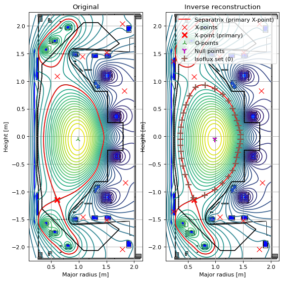
# plot the two equilibria side by side
fig1, (ax1, ax2) = plt.subplots(1, 2, figsize=(8, 8), dpi=80)
for ax, e, title in [(ax1, eq, "Original"), (ax2, eq_inv, "Inverse reconstruction")]:
    ax.grid(True, which="both")
    e.plot(axis=ax, show=False)
    e.tokamak.plot(axis=ax, show=False)
    ax.set_xlim(0.1, 2.15)
    ax.set_ylim(-2.25, 2.25)
    ax.set_title(title)
    if ax == ax2:
        constrain.plot(axis=ax2)
plt.tight_layout()

Coil currents [A]:
      coil      original   reconstructed
  Solenoid        5000.0          4691.0
        PX        3696.8          4125.7
        D1        6941.2          6825.0
        D2        4390.9          4373.9
        D3        2924.4          2899.3
        Dp       -2488.2         -2510.6
        D5         249.2           241.8
        D6        -315.0          -305.5
        D7         511.1           519.2
        P4       -3564.4         -3563.8
        P5       -3954.2         -3971.5
        P6         500.0           508.4

Magnetic axis:   original = [ 0.98617225 -0.051466  ], reconstructed = [ 0.9879268  -0.05120883]
psi_axis:        original = 0.100458, reconstructed = 0.100342
psi_boundary:    original = 0.0314736, reconstructed = 0.031167
Max |Δpsi| relative to max|psi|: 9.579e-03

<Figure size 640x480 with 0 Axes>