Example: linear evolution with re-linearisation during evolutive equilibrium calculations

This notebook also follows on from the previous two.

Here, we demonstrate how to re-calculate the linearisation (e.g. Jacobians) of the dynamics (“relinearise”) when using the linear solver. As we know, the accuracy of the Jacobians (calculated using the initial equilibrium, before evolution) will degrade as the plasma “moves away” from the initial equilibrium around which it was calculated. This means that we need to re-linearise every so often in order to maintain accuracy of the plasma evolution over time.

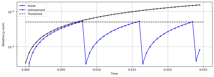
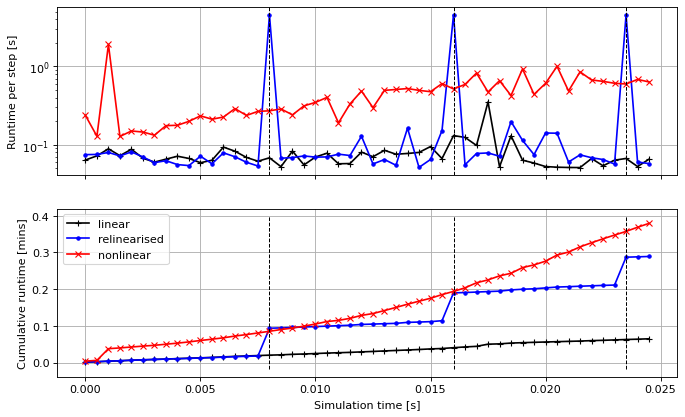
The more often a relinearisation occurs, the more accurate (in theory) a linear simulation will be (when compared to the full nonlinear simulation). It is not practical or efficient to relinearise each timestep, but doing so once a given criterion is met can significantly improve agreement with the nonlinear solver. To trigger relinearisation, we monitor the relative change in plasma current density \(J_{\phi}\) at the current time \(t\) and the initial time \(t_0\). If this threshold exceeds tolerance \(\epsilon\), then we re-linearise around the equilibrium at time \(t\) (and set \(t_0 = t\)).

The criterion checks whether $\( \frac{\left \lVert J_{\phi}(t) - J_{\phi}(t_0) \right \rVert}{\left \lVert J_{\phi}(t_0) \right \rVert} < \epsilon, \)\( is met or not at each timestep \)t$.

Import packages

import numpy as np
import matplotlib.pyplot as plt
from IPython.display import display, clear_output
import pickle
import time

Build the machine

import matplotlib.pyplot as plt
import numpy as np

# build machine
from freegsnke import build_machine
tokamak = build_machine.tokamak(
    active_coils_path=f"../machine_configs/MAST-U/MAST-U_like_active_coils.pickle",
    passive_coils_path=f"../machine_configs/MAST-U/MAST-U_like_passive_coils.pickle",
    limiter_path=f"../machine_configs/MAST-U/MAST-U_like_limiter.pickle",
    wall_path=f"../machine_configs/MAST-U/MAST-U_like_wall.pickle",
)

# initialise equilibrium object
from freegsnke import equilibrium_update
eq = equilibrium_update.Equilibrium(
    tokamak=tokamak,
    Rmin=0.1, Rmax=2.0,   # radial range
    Zmin=-2.2, Zmax=2.2,  # vertical range
    nx=65,                # number of grid points in the radial direction (needs to be of the form (2**n + 1) with n being an integer)
    ny=129,               # number of grid points in the vertical direction (needs to be of the form (2**n + 1) with n being an integer)
    # psi=plasma_psi
)  

# initialise profile object
from freegsnke.jtor_update import ConstrainPaxisIp
profiles = ConstrainPaxisIp(
    eq=eq,
    paxis=8.1e3,
    Ip=6.2e5,
    fvac=0.5,
    alpha_m=1.8,
    alpha_n=1.2
)

# initialise solver
from freegsnke import GSstaticsolver
GSStaticSolver = GSstaticsolver.NKGSsolver(eq)    

# set coil currents
import pickle
with open('data/simple_diverted_currents_PaxisIp.pk', 'rb') as f:
    current_values = pickle.load(f)

for key in current_values.keys():
    eq.tokamak[key].current = current_values[key]

# carry out forward solve
GSStaticSolver.solve(eq=eq, 
                     profiles=profiles, 
                     constrain=None, 
                     target_relative_tolerance=1e-9)

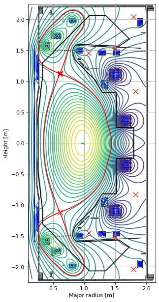
# plot the resulting equilbrium
fig1, ax1 = plt.subplots(1, 1, figsize=(4, 8), dpi=80)
ax1.grid(True, which='both')
eq.plot(axis=ax1, show=False)
eq.tokamak.plot(axis=ax1, show=False)
ax1.set_xlim(0.1, 2.15)
ax1.set_ylim(-2.25, 2.25)
plt.tight_layout()

Active coils --> built from pickle file.
Passive structures --> built from pickle file.
Limiter --> built from pickle file.
Wall --> built from pickle file.

Magnetic probes --> none provided.

Resistance (R) and inductance (M) matrices --> built using actives (and passives if present).
Tokamak built.

Forward static solve SUCCESS. Tolerance 8.76e-10 (vs. requested 1.00e-09) reached in 25/100 iterations.

# define the descriptors function (it should return an array of values and take in an eq object)
def plasma_descriptors(eq):

    # find lower X-point
    # define a "box" in which to search for the lower X-point
    XPT_BOX = [[0.33, -0.88], [0.95, -1.38]]

    # mask those points
    xpt_mask = (
        (eq.xpt[:, 0] >= XPT_BOX[0][0])
        & (eq.xpt[:, 0] <= XPT_BOX[1][0])
        & (eq.xpt[:, 1] <= XPT_BOX[0][1])
        & (eq.xpt[:, 1] >= XPT_BOX[1][1])
    )
    xpts = eq.xpt[xpt_mask, 0:2].squeeze()
    if xpts.ndim > 1 and xpts.shape[0] > 1:
        opt = eq.opt[0, 0:2]
        dists = np.linalg.norm(xpts - opt, axis=1)
        idx = np.argmin(dists)  # index of closest point
        Rx, Zx = xpts[idx, :]
    else:
        Rx, Zx = xpts

    # find avg. Z position of jtor
    Zcurrent = eq.Zcurrent()

    # inboard midplane radius
    Rin = eq.innerOuterSeparatrix()[0]

    return np.array([Zcurrent, Rx, Zx, Rin])

# initialise the nonlinear solver object
from freegsnke import nonlinear_solve

stepping = nonlinear_solve.nl_solver(
    eq=eq, 
    profiles=profiles, 
    GSStaticSolver=GSStaticSolver,
    full_timestep=5e-4, 
    plasma_resistivity=1e-6,
    max_mode_frequency=10**2.5,
    n_linearization_workers=1,  # set >1 to parallelise Jacobian construction
    plasma_descriptor_function=plasma_descriptors
)

-----
Checking that the provided 'eq' and 'profiles' are a GS solution...
Forward static solve SUCCESS. Tolerance 8.76e-10 (vs. requested 1.00e-08) reached in 0/100 iterations.
-----
Instantiating nonlinear solver objects...

done.
-----
Identifying mode selection criteria...
      'threshold_dIy_dI', 'min_dIy_dI', and 'max_mode_frequency' options selected --> passive structure modes are selected according to these thresholds.
-----
Initial mode selection:
   Active coils
      total selected = 12 (out of 12)
   Passive structures
      16 selected below 'max_mode_frequency'
      31 recovered that couple with the plasma more than 'threshold_dIy_dI'
      1 removed that couple with the plasma less than 'min_dIy_dI'
      total selected = 46 (out of 138)
   Total number of modes = 58 (12 active coils + 46 passive structures)
      (Note: some additional modes may be removed after Jacobian calculation)
-----
Building the 3051 x 59 Jacobian (dIy/dI) of plasma current density (inside the LCFS) with respect to all metal currents and the total plasma current.

Building the 3051 x 3 Jacobian (dIy/dtheta) of plasma current density (inside the LCFS) with respect to all plasma current density profile parameters within Jtor.

Built the 4 x 59 Jacobian (ds/dI) of plasma descriptors with respect to all metal currents and the total plasma current.
Built the 4 x 3 Jacobian (ds/dtheta) of plasma descriptors with respect to all plasma current density profile parameters within Jtor.
-----
Further mode reduction:
   1 previously included modes couple with the plasma less than 'min_dIy_dI' (following Jacobian calculation)
   Final number of modes = 57 (12 active coils + 45 passive structures)
   Re-sizing the Jacobian matrix to account for any removed modes (if required).
-----
Stability paramters:

   Deformable plasma metrics:
      Growth rate = [91.85402662] [1/s]
      Instability timescale = [0.01088684] [s]
      Inductive stability margin = [0.5973222+0.j]
   Rigid plasma metrics:
      Leuer parameter (ratio of stabilsing to de-stabilising force gradients):
          between all metals and all metals = 1.7726871416571834
          between all metals and active metals = 1.7726871416571834
          between passive metals and active metals = 1.7726724807891157
-----
Evolutive solver timestep:
      Solver timestep 'dt_step' has been set to 0.0005 as requested.
      Ensure it is smaller than the growth rate else you may find numerical instability in any subsequent evoltuive simulations!
-----

The new n_linearization_workers argument controls how many independent worker processes build both the current-response and profile-parameter-response columns. It applies to the first linearisation constructed by nl_solver and to later relinearisations. The default value of 1 retains the serial calculation. Values larger than one use that many CPU threads in total for Jacobian construction, with one native numerical-library thread per worker to avoid oversubscription. This limit is scoped to Jacobian construction; it does not alter the inner threading used by the ordinary GS solves that advance the evolution.

Carry out standard linear solve

As we have done before, we carry out a standard linear simulation so that we can compare how the relinearisation performs compared to it.

# initialise with the initial condition
stepping.initialize_from_ICs(eq, profiles)

# number of time steps to simulate
max_count = 50

# initialising some variables for iteration and logging
counter = 0
t = 0

history_times = [t]
history_currents = [stepping.currents_vec]
history_equilibria = [stepping.eq1.create_auxiliary_equilibrium()]
history_o_points = [stepping.eq1.opt[0]]
history_elongation = [stepping.eq1.geometricElongation()]
history_triangularity = [stepping.eq1.triangularity()]
history_squareness = [stepping.eq1.squareness()[1]]
history_area = [stepping.eq1.separatrix_area()]
history_length = [stepping.eq1.separatrix_length()]
history_jtor = [stepping.profiles1.jtor]
history_jtor_norm = []
history_timings = []
history_plasma_descriptors = [plasma_descriptors(eq)]

# use constant voltages
voltages = (stepping.vessel_currents_vec*stepping.evol_metal_curr.coil_resist)[:stepping.evol_metal_curr.n_active_coils] 

Call the solver (linear)

We call the linear solver without performing any re-linearisations. This will use the linearisation (calculated when initialize_from_ICs is called) to evolve the plasma for all iterations.

# initialise the solver with the initial equilibrium/profiles
stepping.initialize_from_ICs(eq, profiles)

# loop over time steps
while counter<max_count:
    print(f'Step: {counter}/{max_count-1}')
    print(f'--- t = {t:.2e}')

    # start timer
    start_time = time.time()

    # carry out the time step (profile parameters and resistivity are constant at each time step)
    stepping.nlstepper(
        active_voltage_vec=voltages,   # same voltages used at each time step
        linear_only=True,
        verbose=False,
    )

    # stop timer
    end_time = time.time()

    # store information on the time step
    t += stepping.dt_step
    history_times.append(t)
    counter += 1

    # store time-advanced equilibrium, currents, and profiles (+ other quantites of interest)
    history_currents.append(stepping.currents_vec)
    history_equilibria.append(stepping.eq1.create_auxiliary_equilibrium())
    history_o_points.append(stepping.eq1.opt[0])
    history_elongation.append(stepping.eq1.geometricElongation())
    history_triangularity.append(stepping.eq1.triangularity())
    history_squareness.append(stepping.eq1.squareness()[1])
    history_area.append(stepping.eq1.separatrix_area())
    history_length.append(stepping.eq1.separatrix_length())
    history_jtor.append(stepping.profiles1.jtor)
    history_timings.append(end_time - start_time)
    history_jtor_norm.append(np.linalg.norm(stepping.profiles1.jtor - stepping.jtor0) / np.linalg.norm(stepping.jtor0))
    history_plasma_descriptors.append(plasma_descriptors(stepping.eq1))

# transform lists to arrays
history_currents = np.array(history_currents)
history_times = np.array(history_times)
history_o_points = np.array(history_o_points)
history_elongation = np.array(history_elongation)
history_triangularity = np.array(history_triangularity)
history_squareness = np.array(history_squareness)
history_area = np.array(history_area)
history_length = np.array(history_length)
history_jtor = np.array(history_jtor)
history_timings = np.array(history_timings)
history_jtor_norm = np.array(history_jtor_norm)
history_plasma_descriptors = np.array(history_plasma_descriptors)

Step: 0/49
--- t = 0.00e+00

Step: 1/49
--- t = 5.00e-04

Step: 2/49
--- t = 1.00e-03

Step: 3/49
--- t = 1.50e-03

Step: 4/49
--- t = 2.00e-03

Step: 5/49
--- t = 2.50e-03

Step: 6/49
--- t = 3.00e-03

Step: 7/49
--- t = 3.50e-03

Step: 8/49
--- t = 4.00e-03

Step: 9/49
--- t = 4.50e-03

Step: 10/49
--- t = 5.00e-03

Step: 11/49
--- t = 5.50e-03

Step: 12/49
--- t = 6.00e-03

Step: 13/49
--- t = 6.50e-03

Step: 14/49
--- t = 7.00e-03

Step: 15/49
--- t = 7.50e-03

Step: 16/49
--- t = 8.00e-03

Step: 17/49
--- t = 8.50e-03

Step: 18/49
--- t = 9.00e-03

Step: 19/49
--- t = 9.50e-03

Step: 20/49
--- t = 1.00e-02

Step: 21/49
--- t = 1.05e-02

Step: 22/49
--- t = 1.10e-02

Step: 23/49
--- t = 1.15e-02

Step: 24/49
--- t = 1.20e-02

Step: 25/49
--- t = 1.25e-02

Step: 26/49
--- t = 1.30e-02

Step: 27/49
--- t = 1.35e-02

Step: 28/49
--- t = 1.40e-02

Step: 29/49
--- t = 1.45e-02

Step: 30/49
--- t = 1.50e-02

Step: 31/49
--- t = 1.55e-02

Step: 32/49
--- t = 1.60e-02

Step: 33/49
--- t = 1.65e-02

Step: 34/49
--- t = 1.70e-02

Step: 35/49
--- t = 1.75e-02

Step: 36/49
--- t = 1.80e-02

Step: 37/49
--- t = 1.85e-02

Step: 38/49
--- t = 1.90e-02

Step: 39/49
--- t = 1.95e-02

Step: 40/49
--- t = 2.00e-02

Step: 41/49
--- t = 2.05e-02

Step: 42/49
--- t = 2.10e-02

Step: 43/49
--- t = 2.15e-02

Step: 44/49
--- t = 2.20e-02

Step: 45/49
--- t = 2.25e-02

Step: 46/49
--- t = 2.30e-02

Step: 47/49
--- t = 2.35e-02

Step: 48/49
--- t = 2.40e-02

Step: 49/49
--- t = 2.45e-02

Call the solver (relinearisation)

Again, we evolve the plasma using the linear solver except this time we will provide relinearise_threshold to the nlstepper call (this is the value of \(\epsilon\) we desire). This will re-calculate the linearisation of the dynamics when the relative change in \(J_{\phi}\) is greater than the threshold.

# choose threshold at which to relinearise automatically (this does it at 5%)
threshold = 0.05

# reset the solver object by resetting the initial conditions
stepping.dIydI_ICs = None
stepping.dIydtheta_ICs = None
stepping.initialize_from_ICs(eq, profiles)

# initialising some variables for iteration and logging
counter = 0
t = 0

history_times_rl = [t]
history_currents_rl = [stepping.currents_vec]
history_equilibria_rl = [stepping.eq1.create_auxiliary_equilibrium()]
history_o_points_rl = [stepping.eq1.opt[0]]
history_elongation_rl = [stepping.eq1.geometricElongation()]
history_triangularity_rl = [stepping.eq1.triangularity()]
history_squareness_rl = [stepping.eq1.squareness()[1]]
history_area_rl = [stepping.eq1.separatrix_area()]
history_length_rl = [stepping.eq1.separatrix_length()]
history_timings_rl = []
history_jtor_norm_rl = []
history_plasma_descriptors_rl = [plasma_descriptors(eq)]

# loop over the time steps
while counter<max_count:

    print(f'Step: {counter}/{max_count-1}')
    print(f'--- t = {t:.2e}')
    
    # start timer
    start_time = time.time()

    # carry out the time step
    stepping.nlstepper(
        active_voltage_vec=voltages, 
        linear_only=True,
        verbose=False,
        relinearise_threshold=threshold,
    )

    # stop timer
    end_time = time.time()

    # store information on the time step
    t += stepping.dt_step
    history_times_rl.append(t)
    counter += 1
    
    # store time-advanced equilibrium, currents, and profiles (+ other quantites of interest)
    history_currents_rl.append(stepping.currents_vec)
    history_equilibria_rl.append(stepping.eq1.create_auxiliary_equilibrium())
    history_o_points_rl.append(stepping.eq1.opt[0])
    history_elongation_rl.append(stepping.eq1.geometricElongation())
    history_triangularity_rl.append(stepping.eq1.triangularity())
    history_squareness_rl.append(stepping.eq1.squareness()[1])
    history_area_rl.append(stepping.eq1.separatrix_area())
    history_length_rl.append(stepping.eq1.separatrix_length())
    history_timings_rl.append(end_time - start_time)
    history_jtor_norm_rl.append(stepping.relinearise_criteria)
    history_plasma_descriptors_rl.append(plasma_descriptors(stepping.eq1))

# transform lists to arrays
history_currents_rl = np.array(history_currents_rl)
history_times_rl = np.array(history_times_rl)
history_o_points_rl = np.array(history_o_points_rl)
history_elongation_rl = np.array(history_elongation_rl)
history_triangularity_rl = np.array(history_triangularity_rl)
history_squareness_rl = np.array(history_squareness_rl)
history_area_rl = np.array(history_area_rl)
history_length_rl = np.array(history_length_rl)
history_timings_rl = np.array(history_timings_rl)
history_jtor_norm_rl = np.array(history_jtor_norm_rl)
history_plasma_descriptors_rl = np.array(history_plasma_descriptors_rl)

Building the 3051 x 58 Jacobian (dIy/dI) of plasma current density (inside the LCFS) with respect to all metal currents and the total plasma current.

Building the 3051 x 3 Jacobian (dIy/dtheta) of plasma current density (inside the LCFS) with respect to all plasma current density profile parameters within Jtor.

Built the 4 x 58 Jacobian (ds/dI) of plasma descriptors with respect to all metal currents and the total plasma current.
Built the 4 x 3 Jacobian (ds/dtheta) of plasma descriptors with respect to all plasma current density profile parameters within Jtor.

Step: 0/49
--- t = 0.00e+00

Step: 1/49
--- t = 5.00e-04

Step: 2/49
--- t = 1.00e-03

Step: 3/49
--- t = 1.50e-03

Step: 4/49
--- t = 2.00e-03

Step: 5/49
--- t = 2.50e-03

Step: 6/49
--- t = 3.00e-03

Step: 7/49
--- t = 3.50e-03

Step: 8/49
--- t = 4.00e-03

Step: 9/49
--- t = 4.50e-03

Step: 10/49
--- t = 5.00e-03

Step: 11/49
--- t = 5.50e-03

Step: 12/49
--- t = 6.00e-03

Step: 13/49
--- t = 6.50e-03

Step: 14/49
--- t = 7.00e-03

Step: 15/49
--- t = 7.50e-03

Step: 16/49
--- t = 8.00e-03
Re-linearising around current equilibrium!
   Relative relinearisation criteria change = 5.184% (threshold = 5.0%) 
Building the 3051 x 58 Jacobian (dIy/dI) of plasma current density (inside the LCFS) with respect to all metal currents and the total plasma current.

Building the 3051 x 3 Jacobian (dIy/dtheta) of plasma current density (inside the LCFS) with respect to all plasma current density profile parameters within Jtor.

Built the 4 x 58 Jacobian (ds/dI) of plasma descriptors with respect to all metal currents and the total plasma current.
Built the 4 x 3 Jacobian (ds/dtheta) of plasma descriptors with respect to all plasma current density profile parameters within Jtor.

Step: 17/49
--- t = 8.50e-03

Step: 18/49
--- t = 9.00e-03

Step: 19/49
--- t = 9.50e-03

Step: 20/49
--- t = 1.00e-02

Step: 21/49
--- t = 1.05e-02

Step: 22/49
--- t = 1.10e-02

Step: 23/49
--- t = 1.15e-02

Step: 24/49
--- t = 1.20e-02

Step: 25/49
--- t = 1.25e-02

Step: 26/49
--- t = 1.30e-02

Step: 27/49
--- t = 1.35e-02

Step: 28/49
--- t = 1.40e-02

Step: 29/49
--- t = 1.45e-02

Step: 30/49
--- t = 1.50e-02

Step: 31/49
--- t = 1.55e-02

Step: 32/49
--- t = 1.60e-02
Re-linearising around current equilibrium!
   Relative relinearisation criteria change = 5.199% (threshold = 5.0%) 
Building the 3051 x 58 Jacobian (dIy/dI) of plasma current density (inside the LCFS) with respect to all metal currents and the total plasma current.

Building the 3051 x 3 Jacobian (dIy/dtheta) of plasma current density (inside the LCFS) with respect to all plasma current density profile parameters within Jtor.

Built the 4 x 58 Jacobian (ds/dI) of plasma descriptors with respect to all metal currents and the total plasma current.
Built the 4 x 3 Jacobian (ds/dtheta) of plasma descriptors with respect to all plasma current density profile parameters within Jtor.

Step: 33/49
--- t = 1.65e-02

Step: 34/49
--- t = 1.70e-02

Step: 35/49
--- t = 1.75e-02

Step: 36/49
--- t = 1.80e-02

Step: 37/49
--- t = 1.85e-02

Step: 38/49
--- t = 1.90e-02

Step: 39/49
--- t = 1.95e-02

Step: 40/49
--- t = 2.00e-02

Step: 41/49
--- t = 2.05e-02

Step: 42/49
--- t = 2.10e-02

Step: 43/49
--- t = 2.15e-02

Step: 44/49
--- t = 2.20e-02

Step: 45/49
--- t = 2.25e-02

Step: 46/49
--- t = 2.30e-02

Step: 47/49
--- t = 2.35e-02
Re-linearising around current equilibrium!
   Relative relinearisation criteria change = 5.053% (threshold = 5.0%) 
Building the 3051 x 58 Jacobian (dIy/dI) of plasma current density (inside the LCFS) with respect to all metal currents and the total plasma current.

Building the 3051 x 3 Jacobian (dIy/dtheta) of plasma current density (inside the LCFS) with respect to all plasma current density profile parameters within Jtor.

Built the 4 x 58 Jacobian (ds/dI) of plasma descriptors with respect to all metal currents and the total plasma current.
Built the 4 x 3 Jacobian (ds/dtheta) of plasma descriptors with respect to all plasma current density profile parameters within Jtor.

Step: 48/49
--- t = 2.40e-02

Step: 49/49
--- t = 2.45e-02

Call the solver (nonlinear)

Let us also do a nonlinear simulation to compare the re-linearisation simulation to.

# reset the solver object by resetting the initial conditions
stepping.dIydI_ICs = None
stepping.dIydtheta_ICs = None
stepping.initialize_from_ICs(eq, profiles)

# initialising some variables for iteration and logging
counter = 0
t = 0

history_times_nl = [t]
history_currents_nl = [stepping.currents_vec]
history_equilibria_nl = [stepping.eq1.create_auxiliary_equilibrium()]
history_o_points_nl = [stepping.eq1.opt[0]]
history_elongation_nl = [stepping.eq1.geometricElongation()]
history_triangularity_nl = [stepping.eq1.triangularity()]
history_squareness_nl = [stepping.eq1.squareness()[1]]
history_area_nl = [stepping.eq1.separatrix_area()]
history_length_nl = [stepping.eq1.separatrix_length()]
history_timings_nl = []
history_jtor_norm_nl = []
history_plasma_descriptors_nl = [plasma_descriptors(eq)]

# loop over the time steps
while counter<max_count:

    print(f'Step: {counter}/{max_count-1}')
    print(f'--- t = {t:.2e}')

    # start timer
    start_time = time.time()

    # carry out the time step
    stepping.nlstepper(
        active_voltage_vec=voltages, 
        linear_only=False, 
        verbose=False,
        max_solving_iterations=50,
        target_relative_tol_currents=1e-2,                # relative tolerance in the currents required for convergence
        target_relative_tol_GS=1e-2,                      # relative tolerance in the plasma flux required for convergence
        working_relative_tol_GS=5e-3,                     # tolerance used when solving all static GS problems, expressed in terms of the change in the plasma flux due to 1 timestep of evolution
    )

    # stop timer
    end_time = time.time()
    
    # store information on the time step
    t += stepping.dt_step
    history_times_nl.append(t)
    counter += 1
    
    # store time-advanced equilibrium, currents, and profiles (+ other quantites of interest)
    history_currents_nl.append(stepping.currents_vec)
    history_equilibria_nl.append(stepping.eq1.create_auxiliary_equilibrium())
    history_o_points_nl.append(stepping.eq1.opt[0])
    history_elongation_nl.append(stepping.eq1.geometricElongation())
    history_triangularity_nl.append(stepping.eq1.triangularity())
    history_squareness_nl.append(stepping.eq1.squareness()[1])
    history_area_nl.append(stepping.eq1.separatrix_area())
    history_length_nl.append(stepping.eq1.separatrix_length())
    history_timings_nl.append(end_time - start_time)
    history_jtor_norm_nl.append(stepping.relinearise_criteria)
    history_plasma_descriptors_nl.append(plasma_descriptors(stepping.eq1))

# transform lists to arrays
history_currents_nl = np.array(history_currents_nl)
history_times_nl = np.array(history_times_nl)
history_o_points_nl = np.array(history_o_points_nl)
history_elongation_nl = np.array(history_elongation_nl)
history_triangularity_nl = np.array(history_triangularity_nl)
history_squareness_nl = np.array(history_squareness_nl)
history_area_nl = np.array(history_area_nl)
history_length_nl = np.array(history_length_nl)
history_timings_nl = np.array(history_timings_nl)
history_jtor_norm_nl = np.array(history_jtor_norm_nl)
history_plasma_descriptors_nl = np.array(history_plasma_descriptors_nl)

Building the 3051 x 58 Jacobian (dIy/dI) of plasma current density (inside the LCFS) with respect to all metal currents and the total plasma current.

Building the 3051 x 3 Jacobian (dIy/dtheta) of plasma current density (inside the LCFS) with respect to all plasma current density profile parameters within Jtor.

Built the 4 x 58 Jacobian (ds/dI) of plasma descriptors with respect to all metal currents and the total plasma current.
Built the 4 x 3 Jacobian (ds/dtheta) of plasma descriptors with respect to all plasma current density profile parameters within Jtor.

Step: 0/49
--- t = 0.00e+00

Forward evolutive solve SUCCESS.
   Last max. relative currents change: 6.50e-04 (vs. requested 1.00e-02).
   Last max. relative flux change: 7.57e-03 (vs. requested 1.00e-02).
   Iterations taken: 2/50.

Step: 1/49
--- t = 5.00e-04
Forward evolutive solve SUCCESS.
   Last max. relative currents change: 7.29e-03 (vs. requested 1.00e-02).
   Last max. relative flux change: 3.80e-03 (vs. requested 1.00e-02).
   Iterations taken: 1/50.

Step: 2/49
--- t = 1.00e-03

Forward evolutive solve SUCCESS.
   Last max. relative currents change: 3.76e-03 (vs. requested 1.00e-02).
   Last max. relative flux change: 9.79e-03 (vs. requested 1.00e-02).
   Iterations taken: 2/50.

Step: 3/49
--- t = 1.50e-03
Forward evolutive solve SUCCESS.
   Last max. relative currents change: 9.64e-04 (vs. requested 1.00e-02).
   Last max. relative flux change: 5.66e-03 (vs. requested 1.00e-02).
   Iterations taken: 3/50.

Step: 4/49
--- t = 2.00e-03
Forward evolutive solve SUCCESS.
   Last max. relative currents change: 2.73e-03 (vs. requested 1.00e-02).
   Last max. relative flux change: 3.80e-03 (vs. requested 1.00e-02).
   Iterations taken: 3/50.

Step: 5/49
--- t = 2.50e-03
Forward evolutive solve SUCCESS.
   Last max. relative currents change: 2.50e-03 (vs. requested 1.00e-02).
   Last max. relative flux change: 8.59e-03 (vs. requested 1.00e-02).
   Iterations taken: 4/50.

Step: 6/49
--- t = 3.00e-03
Forward evolutive solve SUCCESS.
   Last max. relative currents change: 1.68e-03 (vs. requested 1.00e-02).
   Last max. relative flux change: 8.37e-03 (vs. requested 1.00e-02).
   Iterations taken: 3/50.

Step: 7/49
--- t = 3.50e-03
Forward evolutive solve SUCCESS.
   Last max. relative currents change: 2.11e-03 (vs. requested 1.00e-02).
   Last max. relative flux change: 4.15e-03 (vs. requested 1.00e-02).
   Iterations taken: 4/50.

Step: 8/49
--- t = 4.00e-03
Forward evolutive solve SUCCESS.
   Last max. relative currents change: 1.73e-03 (vs. requested 1.00e-02).
   Last max. relative flux change: 3.88e-03 (vs. requested 1.00e-02).
   Iterations taken: 4/50.

Step: 9/49
--- t = 4.50e-03
Forward evolutive solve SUCCESS.
   Last max. relative currents change: 9.13e-03 (vs. requested 1.00e-02).
   Last max. relative flux change: 3.90e-03 (vs. requested 1.00e-02).
   Iterations taken: 3/50.

Step: 10/49
--- t = 5.00e-03

Forward evolutive solve SUCCESS.
   Last max. relative currents change: 1.11e-03 (vs. requested 1.00e-02).
   Last max. relative flux change: 3.02e-03 (vs. requested 1.00e-02).
   Iterations taken: 4/50.

Step: 11/49
--- t = 5.50e-03

Forward evolutive solve SUCCESS.
   Last max. relative currents change: 8.40e-03 (vs. requested 1.00e-02).
   Last max. relative flux change: 2.54e-03 (vs. requested 1.00e-02).
   Iterations taken: 3/50.

Step: 12/49
--- t = 6.00e-03

Forward evolutive solve SUCCESS.
   Last max. relative currents change: 6.35e-03 (vs. requested 1.00e-02).
   Last max. relative flux change: 3.64e-03 (vs. requested 1.00e-02).
   Iterations taken: 4/50.

Step: 13/49
--- t = 6.50e-03

Forward evolutive solve SUCCESS.
   Last max. relative currents change: 2.04e-03 (vs. requested 1.00e-02).
   Last max. relative flux change: 6.98e-03 (vs. requested 1.00e-02).
   Iterations taken: 4/50.

Step: 14/49
--- t = 7.00e-03

Forward evolutive solve SUCCESS.
   Last max. relative currents change: 4.99e-03 (vs. requested 1.00e-02).
   Last max. relative flux change: 5.14e-03 (vs. requested 1.00e-02).
   Iterations taken: 4/50.

Step: 15/49
--- t = 7.50e-03

Forward evolutive solve SUCCESS.
   Last max. relative currents change: 6.93e-03 (vs. requested 1.00e-02).
   Last max. relative flux change: 8.25e-03 (vs. requested 1.00e-02).
   Iterations taken: 4/50.

Step: 16/49
--- t = 8.00e-03

Forward evolutive solve SUCCESS.
   Last max. relative currents change: 1.42e-03 (vs. requested 1.00e-02).
   Last max. relative flux change: 6.32e-03 (vs. requested 1.00e-02).
   Iterations taken: 5/50.

Step: 17/49
--- t = 8.50e-03

Forward evolutive solve SUCCESS.
   Last max. relative currents change: 4.39e-03 (vs. requested 1.00e-02).
   Last max. relative flux change: 9.39e-03 (vs. requested 1.00e-02).
   Iterations taken: 5/50.

Step: 18/49
--- t = 9.00e-03

Forward evolutive solve SUCCESS.
   Last max. relative currents change: 9.56e-03 (vs. requested 1.00e-02).
   Last max. relative flux change: 7.33e-03 (vs. requested 1.00e-02).
   Iterations taken: 4/50.

Step: 19/49
--- t = 9.50e-03

Forward evolutive solve SUCCESS.
   Last max. relative currents change: 2.33e-03 (vs. requested 1.00e-02).
   Last max. relative flux change: 8.35e-03 (vs. requested 1.00e-02).
   Iterations taken: 5/50.

Step: 20/49
--- t = 1.00e-02

Forward evolutive solve SUCCESS.
   Last max. relative currents change: 9.65e-04 (vs. requested 1.00e-02).
   Last max. relative flux change: 7.15e-03 (vs. requested 1.00e-02).
   Iterations taken: 7/50.

Step: 21/49
--- t = 1.05e-02

Forward evolutive solve SUCCESS.
   Last max. relative currents change: 1.23e-03 (vs. requested 1.00e-02).
   Last max. relative flux change: 9.99e-03 (vs. requested 1.00e-02).
   Iterations taken: 7/50.

Step: 22/49
--- t = 1.10e-02
Forward evolutive solve SUCCESS.
   Last max. relative currents change: 2.23e-03 (vs. requested 1.00e-02).
   Last max. relative flux change: 7.86e-03 (vs. requested 1.00e-02).
   Iterations taken: 5/50.

Step: 23/49
--- t = 1.15e-02

Forward evolutive solve SUCCESS.
   Last max. relative currents change: 3.51e-03 (vs. requested 1.00e-02).
   Last max. relative flux change: 9.18e-03 (vs. requested 1.00e-02).
   Iterations taken: 5/50.

Step: 24/49
--- t = 1.20e-02

Forward evolutive solve SUCCESS.
   Last max. relative currents change: 3.30e-04 (vs. requested 1.00e-02).
   Last max. relative flux change: 4.35e-03 (vs. requested 1.00e-02).
   Iterations taken: 7/50.

Step: 25/49
--- t = 1.25e-02

Forward evolutive solve SUCCESS.
   Last max. relative currents change: 3.94e-04 (vs. requested 1.00e-02).
   Last max. relative flux change: 8.18e-03 (vs. requested 1.00e-02).
   Iterations taken: 5/50.

Step: 26/49
--- t = 1.30e-02

Forward evolutive solve SUCCESS.
   Last max. relative currents change: 4.35e-03 (vs. requested 1.00e-02).
   Last max. relative flux change: 5.84e-03 (vs. requested 1.00e-02).
   Iterations taken: 5/50.

Step: 27/49
--- t = 1.35e-02

Forward evolutive solve SUCCESS.
   Last max. relative currents change: 6.55e-04 (vs. requested 1.00e-02).
   Last max. relative flux change: 5.67e-03 (vs. requested 1.00e-02).
   Iterations taken: 6/50.

Step: 28/49
--- t = 1.40e-02

Forward evolutive solve SUCCESS.
   Last max. relative currents change: 8.85e-04 (vs. requested 1.00e-02).
   Last max. relative flux change: 5.67e-03 (vs. requested 1.00e-02).
   Iterations taken: 6/50.

Step: 29/49
--- t = 1.45e-02

Forward evolutive solve SUCCESS.
   Last max. relative currents change: 6.36e-03 (vs. requested 1.00e-02).
   Last max. relative flux change: 5.79e-03 (vs. requested 1.00e-02).
   Iterations taken: 5/50.

Step: 30/49
--- t = 1.50e-02

Forward evolutive solve SUCCESS.
   Last max. relative currents change: 1.83e-03 (vs. requested 1.00e-02).
   Last max. relative flux change: 6.27e-03 (vs. requested 1.00e-02).
   Iterations taken: 5/50.

Step: 31/49
--- t = 1.55e-02

Forward evolutive solve SUCCESS.
   Last max. relative currents change: 9.45e-04 (vs. requested 1.00e-02).
   Last max. relative flux change: 5.91e-03 (vs. requested 1.00e-02).
   Iterations taken: 6/50.

Step: 32/49
--- t = 1.60e-02

Forward evolutive solve SUCCESS.
   Last max. relative currents change: 1.70e-03 (vs. requested 1.00e-02).
   Last max. relative flux change: 6.80e-03 (vs. requested 1.00e-02).
   Iterations taken: 5/50.

Step: 33/49
--- t = 1.65e-02

Forward evolutive solve SUCCESS.
   Last max. relative currents change: 2.05e-03 (vs. requested 1.00e-02).
   Last max. relative flux change: 4.68e-03 (vs. requested 1.00e-02).
   Iterations taken: 7/50.

Step: 34/49
--- t = 1.70e-02

Forward evolutive solve SUCCESS.
   Last max. relative currents change: 1.50e-03 (vs. requested 1.00e-02).
   Last max. relative flux change: 9.49e-03 (vs. requested 1.00e-02).
   Iterations taken: 8/50.

Step: 35/49
--- t = 1.75e-02

Forward evolutive solve SUCCESS.
   Last max. relative currents change: 6.36e-03 (vs. requested 1.00e-02).
   Last max. relative flux change: 7.14e-03 (vs. requested 1.00e-02).
   Iterations taken: 5/50.

Step: 36/49
--- t = 1.80e-02

Forward evolutive solve SUCCESS.
   Last max. relative currents change: 2.85e-03 (vs. requested 1.00e-02).
   Last max. relative flux change: 7.64e-03 (vs. requested 1.00e-02).
   Iterations taken: 5/50.

Step: 37/49
--- t = 1.85e-02

Forward evolutive solve SUCCESS.
   Last max. relative currents change: 9.49e-04 (vs. requested 1.00e-02).
   Last max. relative flux change: 7.36e-03 (vs. requested 1.00e-02).
   Iterations taken: 6/50.

Step: 38/49
--- t = 1.90e-02

Forward evolutive solve SUCCESS.
   Last max. relative currents change: 8.25e-04 (vs. requested 1.00e-02).
   Last max. relative flux change: 7.64e-03 (vs. requested 1.00e-02).
   Iterations taken: 6/50.

Step: 39/49
--- t = 1.95e-02

Forward evolutive solve SUCCESS.
   Last max. relative currents change: 4.67e-03 (vs. requested 1.00e-02).
   Last max. relative flux change: 7.37e-03 (vs. requested 1.00e-02).
   Iterations taken: 5/50.

Step: 40/49
--- t = 2.00e-02

Forward evolutive solve SUCCESS.
   Last max. relative currents change: 2.20e-03 (vs. requested 1.00e-02).
   Last max. relative flux change: 7.74e-03 (vs. requested 1.00e-02).
   Iterations taken: 5/50.

Step: 41/49
--- t = 2.05e-02

Forward evolutive solve SUCCESS.
   Last max. relative currents change: 4.76e-04 (vs. requested 1.00e-02).
   Last max. relative flux change: 5.70e-03 (vs. requested 1.00e-02).
   Iterations taken: 7/50.

Step: 42/49
--- t = 2.10e-02

Forward evolutive solve SUCCESS.
   Last max. relative currents change: 2.70e-03 (vs. requested 1.00e-02).
   Last max. relative flux change: 8.98e-03 (vs. requested 1.00e-02).
   Iterations taken: 6/50.

Step: 43/49
--- t = 2.15e-02

Forward evolutive solve SUCCESS.
   Last max. relative currents change: 6.52e-03 (vs. requested 1.00e-02).
   Last max. relative flux change: 6.96e-03 (vs. requested 1.00e-02).
   Iterations taken: 6/50.

Step: 44/49
--- t = 2.20e-02

Forward evolutive solve SUCCESS.
   Last max. relative currents change: 9.68e-03 (vs. requested 1.00e-02).
   Last max. relative flux change: 8.18e-03 (vs. requested 1.00e-02).
   Iterations taken: 6/50.

Step: 45/49
--- t = 2.25e-02

Forward evolutive solve SUCCESS.
   Last max. relative currents change: 1.80e-03 (vs. requested 1.00e-02).
   Last max. relative flux change: 7.94e-03 (vs. requested 1.00e-02).
   Iterations taken: 8/50.

Step: 46/49
--- t = 2.30e-02

Forward evolutive solve SUCCESS.
   Last max. relative currents change: 2.29e-03 (vs. requested 1.00e-02).
   Last max. relative flux change: 8.65e-03 (vs. requested 1.00e-02).
   Iterations taken: 7/50.

Step: 47/49
--- t = 2.35e-02

Forward evolutive solve SUCCESS.
   Last max. relative currents change: 9.84e-03 (vs. requested 1.00e-02).
   Last max. relative flux change: 9.53e-03 (vs. requested 1.00e-02).
   Iterations taken: 6/50.

Step: 48/49
--- t = 2.40e-02

Forward evolutive solve SUCCESS.
   Last max. relative currents change: 4.01e-03 (vs. requested 1.00e-02).
   Last max. relative flux change: 5.10e-03 (vs. requested 1.00e-02).
   Iterations taken: 8/50.

Step: 49/49
--- t = 2.45e-02

Forward evolutive solve SUCCESS.
   Last max. relative currents change: 6.89e-03 (vs. requested 1.00e-02).
   Last max. relative flux change: 9.77e-03 (vs. requested 1.00e-02).
   Iterations taken: 6/50.

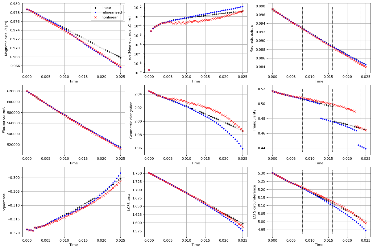
Comparing the simulations

We can now plot a comparison of the nonlinear, linear, and linear (with relinearisation) simulations. We also plot the times at which relinearisation took place (as dashed lines).

We observe performance of the relinearised simulation somewhere “inbetween” the nonlinear and linear simulations as expected! Note that the “jumps” are in the triangularity and the squareness parameters are mostly due to resolution effects.

# Plot evolution of tracked values and compare between linear and non-linear evolution
fig, axs = plt.subplots(3, 3, figsize=(15, 10), dpi=80, constrained_layout=True)
axs_flat = axs.flat

axs_flat[0].plot(history_times, history_o_points[:, 0],'k+', label='linear')
axs_flat[0].plot(history_times_rl, history_o_points_rl[:, 0],'b.', label='relinearised')
axs_flat[0].plot(history_times_nl, history_o_points_nl[:, 0],'rx', label='nonlinear')
axs_flat[0].set_xlabel('Time')
axs_flat[0].set_ylabel('Magnetic axis, $R$ [$m$]')
axs_flat[0].legend()
axs_flat[0].grid()


axs_flat[1].plot(history_times, abs(history_o_points[:, 1]),'k+')
axs_flat[1].plot(history_times_rl, abs(history_o_points_rl[:, 1]),'b.')
axs_flat[1].plot(history_times_nl, abs(history_o_points_nl[:, 1]),'rx')
axs_flat[1].set_yscale('log')
axs_flat[1].set_xlabel('Time')
axs_flat[1].set_ylabel('abs(Magnetic axis, $Z$) [$m$]')
axs_flat[1].grid()

axs_flat[2].plot(history_times, history_o_points[:, 2],'k+')
axs_flat[2].plot(history_times_rl, history_o_points_rl[:, 2],'b.')
axs_flat[2].plot(history_times_nl, history_o_points_nl[:, 2],'rx')
axs_flat[2].set_xlabel('Time')
axs_flat[2].set_ylabel('Magnetic axis, $\psi$')
axs_flat[2].grid()

axs_flat[3].plot(history_times, history_currents[:,-1]*stepping.plasma_norm_factor,'k+')
axs_flat[3].plot(history_times_rl, history_currents_rl[:,-1]*stepping.plasma_norm_factor,'b.')
axs_flat[3].plot(history_times_nl, history_currents_nl[:,-1]*stepping.plasma_norm_factor,'rx')
axs_flat[3].set_xlabel('Time')
axs_flat[3].set_ylabel('Plasma current')
axs_flat[3].grid()

axs_flat[4].plot(history_times, history_elongation,'k+')
axs_flat[4].plot(history_times_rl, history_elongation_rl,'b.')
axs_flat[4].plot(history_times_nl, history_elongation_nl,'rx')
axs_flat[4].set_xlabel('Time')
axs_flat[4].set_ylabel('Geometric elongation')
axs_flat[4].grid()

axs_flat[5].plot(history_times, history_triangularity,'k+')
axs_flat[5].plot(history_times_rl, history_triangularity_rl,'b.')
axs_flat[5].plot(history_times_nl, history_triangularity_nl,'rx')
axs_flat[5].set_xlabel('Time')
axs_flat[5].set_ylabel('Triangularity')
axs_flat[5].grid()

axs_flat[6].plot(history_times, history_squareness,'k+')
axs_flat[6].plot(history_times_rl, history_squareness_rl,'b.')
axs_flat[6].plot(history_times_nl, history_squareness_nl,'rx')
axs_flat[6].set_xlabel('Time')
axs_flat[6].set_ylabel('Squarenss')
axs_flat[6].grid()

axs_flat[7].plot(history_times, history_area,'k+')
axs_flat[7].plot(history_times_rl, history_area_rl,'b.')
axs_flat[7].plot(history_times_nl, history_area_nl,'rx')
axs_flat[7].set_xlabel('Time')
axs_flat[7].set_ylabel('LCFS area')
axs_flat[7].grid()

axs_flat[8].plot(history_times, history_length,'k+')
axs_flat[8].plot(history_times_rl, history_length_rl,'b.')
axs_flat[8].plot(history_times_nl, history_length_nl,'rx')
axs_flat[8].set_xlabel('Time')
axs_flat[8].set_ylabel('LCFS circumference')
axs_flat[8].grid()


# plot relinearisation times
relin_times = history_times_rl[0:-1][history_jtor_norm_rl > threshold]
for i in range(0,9):
    axs_flat[i].vlines(relin_times, ymin=[axs_flat[i].get_ylim()[0]]*len(relin_times), ymax=[axs_flat[i].get_ylim()[1]]*len(relin_times), linestyles="--", color="k", linewidths=0.7)

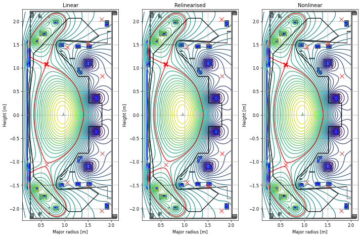
# plot the equilibria at the final time step
fig1, (ax1, ax2, ax3) = plt.subplots(1, 3, figsize=(12, 8), dpi=60)

ax1.grid(True, which='both')
history_equilibria[-1].plot(axis=ax1, show=False)
eq.tokamak.plot(axis=ax1, show=False)
ax1.set_xlim(0.1, 2.15)
ax1.set_ylim(-2.25, 2.25)
ax1.set_title("Linear")

ax2.grid(True, which='both')
history_equilibria_rl[-1].plot(axis=ax2, show=False)
eq.tokamak.plot(axis=ax2, show=False)
ax2.set_xlim(0.1, 2.15)
ax2.set_ylim(-2.25, 2.25)
ax2.set_title("Relinearised")

ax3.grid(True, which='both')
history_equilibria_nl[-1].plot(axis=ax3, show=False)
eq.tokamak.plot(axis=ax3, show=False)
ax3.set_xlim(0.1, 2.15)
ax3.set_ylim(-2.25, 2.25)
ax3.set_title("Nonlinear")

plt.tight_layout()

# plot relinearisation criteria evolution
fig, axs = plt.subplots(1, 1, figsize=(12, 4), dpi=80)
axs.plot(history_times[0:-1], history_jtor_norm, 'k+-', label="linear")
axs.plot(history_times_rl[0:-1], history_jtor_norm_rl, 'b.-', label="relinearised")
axs.hlines(threshold, xmin=history_times[0], xmax=history_times[-1], linestyle='--', color='k', label="Threshold")
axs.set_xlabel('Time')
axs.set_ylabel(r"Relative $J_{\phi}$ norm")
axs.set_yscale('log')
axs.legend()
axs.grid()

# plot runtimes
fig, axs = plt.subplots(2, 1, figsize=(10, 6), dpi=80)
axs = axs.flat

axs[0].plot(history_times[0:-1], history_timings, 'k+-', label="linear")
axs[0].plot(history_times_rl[0:-1], history_timings_rl, 'b.-', label="relinearised")
axs[0].plot(history_times_nl[0:-1], history_timings_nl, 'rx-', label="nonlinear")
axs[0].set_ylabel('Runtime per step [s]')
axs[0].set_yscale('log')
axs[0].grid()
axs[0].set_xticklabels([])

axs[1].plot(history_times[0:-1], np.cumsum(history_timings)/60, 'k+-', label="linear")
axs[1].plot(history_times_rl[0:-1], np.cumsum(history_timings_rl)/60, 'b.-', label="relinearised")
axs[1].plot(history_times_nl[0:-1], np.cumsum(history_timings_nl)/60, 'rx-', label="nonlinear")


# plot relinearisation times
for i in range(0,2):
    axs[i].vlines(relin_times, ymin=[axs[i].get_ylim()[0]]*len(relin_times), ymax=[axs[i].get_ylim()[1]]*len(relin_times), linestyles="--", color="k", linewidths=0.9)

# axs.plot(jtor_norm_nl)
axs[1].set_xlabel('Simulation time [s]')
axs[1].set_ylabel('Cumulative runtime [mins]')
axs[1].legend()
axs[1].grid()

Re-linearising when using the no_GS option

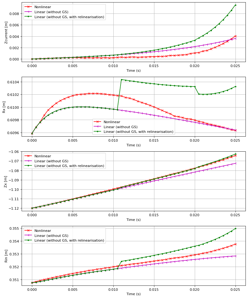
Next, we will do the same simulations (with and without relinearisation) but this time without solving Grad-Shafranov at each timestep (see prior example notebook). This will enable a very fast simulation but, due to the lack of a control scheme, the accuracy of the simulation will be lost very quickly (less so when relinearisation is switched on).

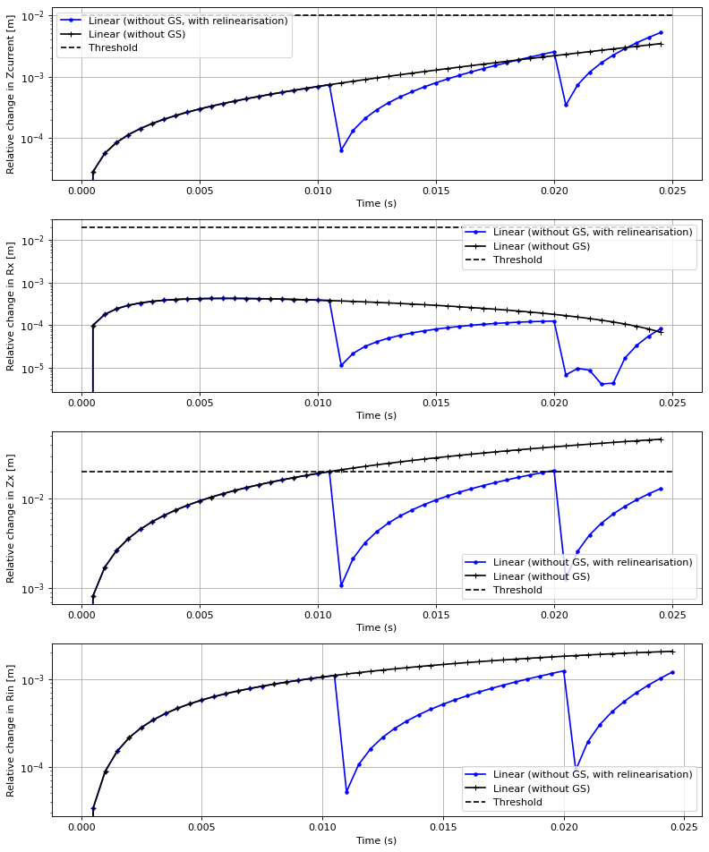
We should note that given GS is no longer solved, the criterion for relinearisation is no longer valid (as we will not have access to \(J_{\phi}\) at each timestep). We therefore carry out relinearisation when the absolute change in the plasma_descriptors (with respect to the values at the last linearisation) exceeds \(\epsilon\).

A value for \(\epsilon\) can be set for each descriptor individually (as a list of floats) or for all of them (as a single float).

First let us carry out a standard linear simulation without solving GS at each timestep (no relinearisation is carried out). Here we set the relinearise_threshold as a list of None (or large) values to indicate that we do not relinearise at all.

# reset the solver object by resetting the initial conditions
stepping.dIydI_ICs = None
stepping.dIydtheta_ICs = None
stepping.initialize_from_ICs(eq, profiles)

counter = 0
t = 0

# storage
history_times_nogs = [t]
history_currents_nogs = [stepping.currents_vec]
history_plasma_descriptors_nogs = [plasma_descriptors(eq)]
history_criteria_nogs = []

Building the 3051 x 58 Jacobian (dIy/dI) of plasma current density (inside the LCFS) with respect to all metal currents and the total plasma current.

Building the 3051 x 3 Jacobian (dIy/dtheta) of plasma current density (inside the LCFS) with respect to all plasma current density profile parameters within Jtor.

Built the 4 x 58 Jacobian (ds/dI) of plasma descriptors with respect to all metal currents and the total plasma current.
Built the 4 x 3 Jacobian (ds/dtheta) of plasma descriptors with respect to all plasma current density profile parameters within Jtor.

# simulate
while counter < max_count:
    print(f'Step: {counter}/{max_count-1}')
    print(f'--- t = {t:.2e}')

    # carry out the time step (feed in the voltages and profile parameters)
    stepping.nlstepper(
        active_voltage_vec=voltages,
        linear_only=True,
        no_GS=True,
        verbose=False,
        relinearise_threshold=[None, 1.0, 1.0, 1.0],
    )

    # store time-advanced currents and plasma descriptors
    history_currents_nogs.append(stepping.currents_vec)
    history_plasma_descriptors_nogs.append(stepping.plasma_descriptors_vec)
    history_criteria_nogs.append(stepping.relinearise_criteria)

    t += stepping.dt_step
    history_times_nogs.append(t)
    counter += 1

# transform lists to arrays
history_currents_nogs = np.array(history_currents_nogs)
history_times_nogs = np.array(history_times_nogs)
history_plasma_descriptors_nogs = np.array(history_plasma_descriptors_nogs)
history_criteria_nogs = np.array(history_criteria_nogs)

Step: 0/49
--- t = 0.00e+00
Step: 1/49
--- t = 5.00e-04
Step: 2/49
--- t = 1.00e-03
Step: 3/49
--- t = 1.50e-03
Step: 4/49
--- t = 2.00e-03
Step: 5/49
--- t = 2.50e-03
Step: 6/49
--- t = 3.00e-03
Step: 7/49
--- t = 3.50e-03
Step: 8/49
--- t = 4.00e-03
Step: 9/49
--- t = 4.50e-03
Step: 10/49
--- t = 5.00e-03
Step: 11/49
--- t = 5.50e-03
Step: 12/49
--- t = 6.00e-03
Step: 13/49
--- t = 6.50e-03
Step: 14/49
--- t = 7.00e-03
Step: 15/49
--- t = 7.50e-03
Step: 16/49
--- t = 8.00e-03
Step: 17/49
--- t = 8.50e-03
Step: 18/49
--- t = 9.00e-03
Step: 19/49
--- t = 9.50e-03
Step: 20/49
--- t = 1.00e-02
Step: 21/49
--- t = 1.05e-02
Step: 22/49
--- t = 1.10e-02
Step: 23/49
--- t = 1.15e-02
Step: 24/49
--- t = 1.20e-02
Step: 25/49
--- t = 1.25e-02

Step: 26/49
--- t = 1.30e-02
Step: 27/49
--- t = 1.35e-02
Step: 28/49
--- t = 1.40e-02
Step: 29/49
--- t = 1.45e-02
Step: 30/49
--- t = 1.50e-02
Step: 31/49
--- t = 1.55e-02
Step: 32/49
--- t = 1.60e-02
Step: 33/49
--- t = 1.65e-02
Step: 34/49
--- t = 1.70e-02
Step: 35/49
--- t = 1.75e-02
Step: 36/49
--- t = 1.80e-02
Step: 37/49
--- t = 1.85e-02
Step: 38/49
--- t = 1.90e-02
Step: 39/49
--- t = 1.95e-02
Step: 40/49
--- t = 2.00e-02
Step: 41/49
--- t = 2.05e-02
Step: 42/49
--- t = 2.10e-02
Step: 43/49
--- t = 2.15e-02
Step: 44/49
--- t = 2.20e-02
Step: 45/49
--- t = 2.25e-02
Step: 46/49
--- t = 2.30e-02
Step: 47/49
--- t = 2.35e-02

Step: 48/49
--- t = 2.40e-02
Step: 49/49
--- t = 2.45e-02

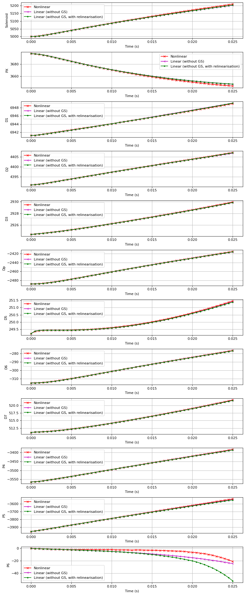
Next, we’ll do the same simulation but this time we will enable re-linearisation when one of the shape parameter changes exceeds a few centimetres.

# reset the solver object by resetting the initial conditions
stepping.dIydI_ICs = None
stepping.dIydtheta_ICs = None
stepping.initialize_from_ICs(eq, profiles)

counter = 0
t = 0

# storage
history_times_nogs_rl = [t]
history_currents_nogs_rl = [stepping.currents_vec]
history_plasma_descriptors_nogs_rl = [plasma_descriptors(eq)]
history_criteria_nogs_rl = []

Building the 3051 x 58 Jacobian (dIy/dI) of plasma current density (inside the LCFS) with respect to all metal currents and the total plasma current.

Building the 3051 x 3 Jacobian (dIy/dtheta) of plasma current density (inside the LCFS) with respect to all plasma current density profile parameters within Jtor.

Built the 4 x 58 Jacobian (ds/dI) of plasma descriptors with respect to all metal currents and the total plasma current.
Built the 4 x 3 Jacobian (ds/dtheta) of plasma descriptors with respect to all plasma current density profile parameters within Jtor.

# simulate
thresholds = [0.01, 0.02, 0.02, None]

currents = []
profs = []
params = []
while counter < max_count:
    print(f'Step: {counter}/{max_count-1}')
    print(f'--- t = {t:.2e}')

    # carry out the time step (feed in the voltages and profile parameters)
    stepping.nlstepper(
        active_voltage_vec=voltages,
        linear_only=True,
        no_GS=True,
        verbose=False,
        relinearise_threshold=thresholds,
    )

    # store time-advanced currents and plasma descriptors
    history_currents_nogs_rl.append(stepping.currents_vec)
    history_plasma_descriptors_nogs_rl.append(stepping.plasma_descriptors_vec)
    history_criteria_nogs_rl.append(stepping.relinearise_criteria)

    t += stepping.dt_step
    history_times_nogs_rl.append(t)
    counter += 1

    currents.append(stepping.initial_currents_plasma_descriptor)
    profs.append(stepping.initial_profiles_plasma_descriptor)   
    params.append(stepping.initial_plasma_descriptors)

# transform lists to arrays
history_currents_nogs_rl = np.array(history_currents_nogs_rl)
history_times_nogs_rl = np.array(history_times_nogs_rl)
history_plasma_descriptors_nogs_rl = np.array(history_plasma_descriptors_nogs_rl)
history_criteria_nogs_rl = np.array(history_criteria_nogs_rl)

Step: 0/49
--- t = 0.00e+00
Step: 1/49
--- t = 5.00e-04
Step: 2/49
--- t = 1.00e-03
Step: 3/49
--- t = 1.50e-03
Step: 4/49
--- t = 2.00e-03
Step: 5/49
--- t = 2.50e-03
Step: 6/49
--- t = 3.00e-03
Step: 7/49
--- t = 3.50e-03
Step: 8/49
--- t = 4.00e-03
Step: 9/49
--- t = 4.50e-03
Step: 10/49
--- t = 5.00e-03
Step: 11/49
--- t = 5.50e-03
Step: 12/49
--- t = 6.00e-03
Step: 13/49
--- t = 6.50e-03
Step: 14/49
--- t = 7.00e-03
Step: 15/49
--- t = 7.50e-03
Step: 16/49
--- t = 8.00e-03
Step: 17/49
--- t = 8.50e-03
Step: 18/49
--- t = 9.00e-03
Step: 19/49
--- t = 9.50e-03
Step: 20/49
--- t = 1.00e-02
Step: 21/49
--- t = 1.05e-02
Re-linearising around current equilibrium!

   Absolute relinearisation criteria change = [0.001 0.    0.02  0.001] (threshold = [0.01 0.02 0.02  inf]) 
Building the 3051 x 58 Jacobian (dIy/dI) of plasma current density (inside the LCFS) with respect to all metal currents and the total plasma current.

Building the 3051 x 3 Jacobian (dIy/dtheta) of plasma current density (inside the LCFS) with respect to all plasma current density profile parameters within Jtor.

Built the 4 x 58 Jacobian (ds/dI) of plasma descriptors with respect to all metal currents and the total plasma current.
Built the 4 x 3 Jacobian (ds/dtheta) of plasma descriptors with respect to all plasma current density profile parameters within Jtor.
Step: 22/49
--- t = 1.10e-02
Step: 23/49
--- t = 1.15e-02
Step: 24/49
--- t = 1.20e-02
Step: 25/49
--- t = 1.25e-02
Step: 26/49
--- t = 1.30e-02
Step: 27/49
--- t = 1.35e-02
Step: 28/49
--- t = 1.40e-02
Step: 29/49
--- t = 1.45e-02
Step: 30/49
--- t = 1.50e-02
Step: 31/49
--- t = 1.55e-02
Step: 32/49
--- t = 1.60e-02
Step: 33/49
--- t = 1.65e-02
Step: 34/49
--- t = 1.70e-02
Step: 35/49
--- t = 1.75e-02
Step: 36/49
--- t = 1.80e-02
Step: 37/49
--- t = 1.85e-02
Step: 38/49
--- t = 1.90e-02
Step: 39/49
--- t = 1.95e-02
Step: 40/49
--- t = 2.00e-02
Re-linearising around current equilibrium!

   Absolute relinearisation criteria change = [0.003 0.    0.021 0.001] (threshold = [0.01 0.02 0.02  inf]) 
Building the 3051 x 58 Jacobian (dIy/dI) of plasma current density (inside the LCFS) with respect to all metal currents and the total plasma current.

Building the 3051 x 3 Jacobian (dIy/dtheta) of plasma current density (inside the LCFS) with respect to all plasma current density profile parameters within Jtor.

Built the 4 x 58 Jacobian (ds/dI) of plasma descriptors with respect to all metal currents and the total plasma current.
Built the 4 x 3 Jacobian (ds/dtheta) of plasma descriptors with respect to all plasma current density profile parameters within Jtor.
Step: 41/49
--- t = 2.05e-02
Step: 42/49
--- t = 2.10e-02
Step: 43/49
--- t = 2.15e-02
Step: 44/49
--- t = 2.20e-02
Step: 45/49
--- t = 2.25e-02
Step: 46/49
--- t = 2.30e-02
Step: 47/49
--- t = 2.35e-02
Step: 48/49
--- t = 2.40e-02
Step: 49/49
--- t = 2.45e-02

fig, ax = plt.subplots(4,1, figsize=(10, 12), dpi=80)
ax = ax.flatten()

labels = ["Zcurrent [m]", "Rx [m]", "Zx [m]", "Rin [m]"]

for i in range(4):
    ax[i].plot(history_times, history_plasma_descriptors_nl[:, i], 'rx-', label="Nonlinear")
    # ax[i].plot(history_times, history_plasma_descriptors[:, i], 'k+-', label="Linear (with GS)")
    ax[i].plot(history_times_nogs, history_plasma_descriptors_nogs[:, i], 'm3-', label="Linear (without GS)")
    ax[i].plot(history_times_nogs_rl, history_plasma_descriptors_nogs_rl[:, i], 'g.-', label="Linear (without GS, with relinearisation)")
    ax[i].set_xlabel("Time (s)")
    ax[i].set_ylabel(labels[i])
    ax[i].legend()
    ax[i].grid()

fig.tight_layout()

# plot relinearisation criteria evolution
fig, ax = plt.subplots(4,1, figsize=(10, 12), dpi=80)
ax = ax.flatten()

for i in range(4):
    ax[i].plot(history_times_nogs_rl[0:-1], history_criteria_nogs_rl[:, i], 'b.-', label="Linear (without GS, with relinearisation)")
    ax[i].plot(history_times_nogs[0:-1], history_criteria_nogs[:, i], 'k+-', label="Linear (without GS)")
    ax[i].hlines(thresholds[i], xmin=history_times_nogs_rl[0], xmax=history_times_nogs_rl[-1], linestyle='--', color='k', label="Threshold")
    ax[i].set_xlabel("Time (s)")
    ax[i].set_ylabel(f"Relative change in {labels[i]}")
    ax[i].set_yscale('log')
    ax[i].legend()
    ax[i].grid()

fig.tight_layout()


# fig, axs = plt.subplots(1, 1, figsize=(12, 4), dpi=80)
# # axs.plot(history_times_nogs[0:-1], history_jtor_norm, 'k+-', label="linear")
# axs.plot(history_times_nogs[0:-1], history_criteria_nogs, 'b.-', label="relinearised")
# axs.hlines(threshold, xmin=history_times[0], xmax=history_times[-1], linestyle='--', color='k', label="Threshold")
# axs.set_xlabel('Time')
# axs.set_ylabel(r"Relative $J_{\phi}$ norm")
# axs.set_yscale('log')
# axs.legend()
# axs.grid()

fig, ax = plt.subplots(12,1, figsize=(10, 24), dpi=80)
ax = ax.flatten()

labels = eq.tokamak.coil_names[0:12]

for i in range(len(labels)):
    ax[i].plot(history_times, history_currents_nl[:, i], 'rx-', label="Nonlinear")
    # ax[i].plot(history_times, history_plasma_descriptors[:, i], 'k+-', label="Linear (with GS)")
    ax[i].plot(history_times_nogs, history_currents_nogs[:, i], 'm3-', label="Linear (without GS)")
    ax[i].plot(history_times_nogs_rl, history_currents_nogs_rl[:, i], 'g.-', label="Linear (without GS, with relinearisation)")
    ax[i].set_xlabel("Time (s)")
    ax[i].set_ylabel(labels[i])
    ax[i].legend()
    ax[i].grid()

fig.tight_layout()