Example: linear evolution without solving the Grad-Shafranov equation
This notebook follows on from the previous one, except that the following (linear) evolutive solves will not solve the GS equation at each timestep.
This mode uses the linearisations from the initial equilibrium configuration at time \(t=0\) (i.e. the Jacobians inside the evolutive solver) to evolve plasma shape parameters of interest (e.g. midplane radii, X-point positions) forward in time rapidly.
This can be useful for doing very fast scans forward in time into how certain shape parameters will evolve (linearly at least). Note, however, the equilibria for these simulations cannot be visualised as GS has not been solved!
The simulation proceeds in almost exactly the same way as the previous notebook so please do check that out first.
Static forward simulation
Begin by building the initial plasma configuration as usual.
import matplotlib.pyplot as plt
import numpy as np

# build machine
from freegsnke import build_machine
tokamak = build_machine.tokamak(
    active_coils_path=f"../machine_configs/MAST-U/MAST-U_like_active_coils.pickle",
    passive_coils_path=f"../machine_configs/MAST-U/MAST-U_like_passive_coils.pickle",
    limiter_path=f"../machine_configs/MAST-U/MAST-U_like_limiter.pickle",
    wall_path=f"../machine_configs/MAST-U/MAST-U_like_wall.pickle",
)

# initialise equilibrium object
from freegsnke import equilibrium_update
eq = equilibrium_update.Equilibrium(
    tokamak=tokamak,
    Rmin=0.1, Rmax=2.0,   # radial range
    Zmin=-2.2, Zmax=2.2,  # vertical range
    nx=65,                # number of grid points in the radial direction (needs to be of the form (2**n + 1) with n being an integer)
    ny=129,               # number of grid points in the vertical direction (needs to be of the form (2**n + 1) with n being an integer)
    # psi=plasma_psi
)

# initialise profile object
from freegsnke.jtor_update import ConstrainPaxisIp
profiles = ConstrainPaxisIp(
    eq=eq,
    paxis=8.1e3,
    Ip=6.2e5,
    fvac=0.5,
    alpha_m=1.8,
    alpha_n=1.2
)

# initialise solver
from freegsnke import GSstaticsolver
GSStaticSolver = GSstaticsolver.NKGSsolver(eq)

# set coil currents
import pickle
with open('data/simple_diverted_currents_PaxisIp.pk', 'rb') as f:
    current_values = pickle.load(f)

for key in current_values.keys():
    eq.tokamak[key].current = current_values[key]
eq.tokamak["P6"].current += 100

# carry out forward solve
GSStaticSolver.solve(eq=eq,
                     profiles=profiles,
                     constrain=None,
                     target_relative_tolerance=1e-9)

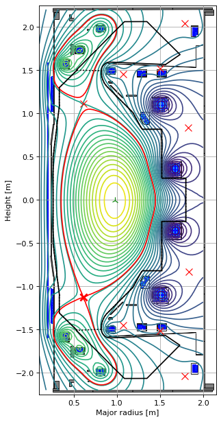
# plot the resulting equilbrium
fig1, ax1 = plt.subplots(1, 1, figsize=(4, 8), dpi=80)
ax1.grid(True, which='both')
eq.plot(axis=ax1, show=False)
eq.tokamak.plot(axis=ax1, show=False)
ax1.set_xlim(0.1, 2.15)
ax1.set_ylim(-2.25, 2.25)
plt.tight_layout()
Active coils --> built from pickle file.
Passive structures --> built from pickle file.
Limiter --> built from pickle file.
Wall --> built from pickle file.
Magnetic probes --> none provided.
Resistance (R) and inductance (M) matrices --> built using actives (and passives if present).
Tokamak built.
Forward static solve SUCCESS. Tolerance 1.93e-10 (vs. requested 1.00e-09) reached in 24/100 iterations.
Define the plasma descriptors
Here we define the “plasma descriptors” (i.e. the shape parameters) that we want to track over time. These descriptors will be evolved according to the following equation:
where
\(\vec{s}(t)\) are the plasma descriptors (defined in the following cells) approximated via the linearisation, and \(\vec{s}(0)\) are the values defined by the initial equilibrium configuration.
\(\vec{I}_e(t) = (\vec{I}_m(t), I_p(t))\) is a vector of the currents in the metals and total plasma current at time \(t\).
\(\vec{\theta}(t)\) are the (plasma current density) profile parameters at time \(t\).
\(\frac{\partial \vec{s}}{\partial \vec{I}_e}\) and \(\frac{\partial \vec{s}}{\partial \vec{\theta}}\) are the Jacobians calculated wrt the initial equilibrium.
The currents come from solving the circuit equations the same way as before while the plasma profile parameters are inputs provided by the user.
This enables a rapid (approximate) evolution of these descriptors over short periods of time - noting that the Jacobians lose accuracy as they diverge from the equilibrium from which they were constructed.
The plasma descriptors are defined via a function that must take a FreeGSNKE equilibrium object as its sole input.
For example, below we define a function that will return an array containing: the average \(Z\) position of the \(J_{\phi}\) map; the radial and vertical position of the lower X-point; and the inboard midplane radius.
This can be customised to add any descriptors of interest to you.
# define the descriptors function (it should return an array of values and take in an eq object)
def plasma_descriptors(eq):

    # find lower X-point
    # define a "box" in which to search for the lower X-point
    XPT_BOX = [[0.33, -0.88], [0.95, -1.38]]

    # mask those points
    xpt_mask = (
        (eq.xpt[:, 0] >= XPT_BOX[0][0])
        & (eq.xpt[:, 0] <= XPT_BOX[1][0])
        & (eq.xpt[:, 1] <= XPT_BOX[0][1])
        & (eq.xpt[:, 1] >= XPT_BOX[1][1])
    )
    xpts = eq.xpt[xpt_mask, 0:2].squeeze()
    if xpts.ndim > 1 and xpts.shape[0] > 1:
        opt = eq.opt[0, 0:2]
        dists = np.linalg.norm(xpts - opt, axis=1)
        idx = np.argmin(dists)  # index of closest point
        Rx, Zx = xpts[idx, :]
    else:
        Rx, Zx = xpts

    # find avg. Z position of jtor
    Zcurrent = eq.Zcurrent()

    # inboard midplane radius
    Rin = eq.innerOuterSeparatrix()[0]

    return np.array([Zcurrent, Rx, Zx, Rin])
Time evolution
Having defined the plasma descriptors, we can now instantiate the evolutive solver object. By including the plasma_descriptors function as an argument, the relevant Jacobians will be calculated to enable this evolution.
The new n_linearization_workers argument controls the number of independent worker processes used to construct both the current-response and profile-parameter-response Jacobian columns. 1 retains serial construction; a larger value parallelises the initial linearisation and any later relinearisations. It does not limit the inner threading of ordinary time-step GS solves.
from freegsnke import nonlinear_solve

stepping = nonlinear_solve.nl_solver(
    eq=eq,
    profiles=profiles,
    GSStaticSolver=GSStaticSolver,
    full_timestep=5e-4,
    plasma_resistivity=1e-6,
    max_mode_frequency=10**2.5,
    n_linearization_workers=1,  # set >1 to parallelise Jacobian construction
    plasma_descriptor_function=plasma_descriptors
)
-----
Checking that the provided 'eq' and 'profiles' are a GS solution...
Forward static solve SUCCESS. Tolerance 1.93e-10 (vs. requested 1.00e-08) reached in 0/100 iterations.
-----
Instantiating nonlinear solver objects...
done.
-----
Identifying mode selection criteria...
      'threshold_dIy_dI', 'min_dIy_dI', and 'max_mode_frequency' options selected --> passive structure modes are selected according to these thresholds.
-----
Initial mode selection:
   Active coils
      total selected = 12 (out of 12)
   Passive structures
      16 selected below 'max_mode_frequency'
      31 recovered that couple with the plasma more than 'threshold_dIy_dI'
      1 removed that couple with the plasma less than 'min_dIy_dI'
      total selected = 46 (out of 138)
   Total number of modes = 58 (12 active coils + 46 passive structures)
      (Note: some additional modes may be removed after Jacobian calculation)
-----
Building the 3051 x 59 Jacobian (dIy/dI) of plasma current density (inside the LCFS) with respect to all metal currents and the total plasma current.
Building the 3051 x 3 Jacobian (dIy/dtheta) of plasma current density (inside the LCFS) with respect to all plasma current density profile parameters within Jtor.
Built the 4 x 59 Jacobian (ds/dI) of plasma descriptors with respect to all metal currents and the total plasma current.
Built the 4 x 3 Jacobian (ds/dtheta) of plasma descriptors with respect to all plasma current density profile parameters within Jtor.
-----
Further mode reduction:
   1 previously included modes couple with the plasma less than 'min_dIy_dI' (following Jacobian calculation)
   Final number of modes = 57 (12 active coils + 45 passive structures)
   Re-sizing the Jacobian matrix to account for any removed modes (if required).
-----
Stability paramters:
   Deformable plasma metrics:
      Growth rate = [77.56183481] [1/s]
      Instability timescale = [0.01289294] [s]
      Inductive stability margin = [0.63236597+0.j]
   Rigid plasma metrics:
      Leuer parameter (ratio of stabilsing to de-stabilising force gradients):
          between all metals and all metals = 1.7926165142473538
          between all metals and active metals = 1.7926165142473538
          between passive metals and active metals = 1.7926023427473192
-----
Evolutive solver timestep:
      Solver timestep 'dt_step' has been set to 0.0005 as requested.
      Ensure it is smaller than the growth rate else you may find numerical instability in any subsequent evoltuive simulations!
-----
Carry out time stepping
As we did in the previous notebook, we define the number of steps we wish to take (based on the timestep chosen above) and create some storage lists.
# number of time steps to simulate
max_count = 50

# initialising some variables for iteration and logging
counter = 0
t = 0

# initialise object
stepping.initialize_from_ICs(eq, profiles)

# storage
history_times = [t]
history_currents = [stepping.currents_vec]
history_plasma_descriptors = [plasma_descriptors(eq)]
# constant voltages (i.e. no control or external drive)
voltages = (stepping.vessel_currents_vec*stepping.evol_metal_curr.coil_resist)[:stepping.evol_metal_curr.n_active_coils]

# # time-dependent plasma current density profile parameters
# alpha_m = np.tile(profiles.alpha_m, max_count+1)
# alpha_m -= (0.1 * np.sin(0.05 * np.pi * np.arange(max_count+1))) # we add some perturbation

# alpha_n = np.tile(profiles.alpha_n, max_count+1)
# alpha_n += (0.1 * np.sin(0.1 * np.pi * np.arange(max_count+1))) # we add some perturbation

# paxis = np.tile(profiles.paxis, max_count+1)
# paxis += (0.1 * np.sin(0.01 * np.pi * np.arange(max_count+1))) # we add some perturbation
We can now call the timestepper with both the linear_only=True and no_GS=True options. This ensures that a linear solve is carried out without solving GS at each timestep. Note that you will not be able to extract all of the usual equilibrium information at each timestep as the internal eq objects no longer contain valid GS solutions! Switch back to no_GS=False if that’s what you need.
This means that in this mode of evolution, only the the metal currents, the plasma current, and the plasma descriptors are evolved over time.
# loop over time steps
while counter < max_count:
    print(f'Step: {counter}/{max_count-1}')
    print(f'--- t = {t:.2e}')

    # carry out the time step (feed in the voltages and profile parameters)
    stepping.nlstepper(
        active_voltage_vec=voltages,
        linear_only=True,
        no_GS=True,
        verbose=False,
    )

    # store time-advanced currents and plasma descriptors
    history_currents.append(stepping.currents_vec)
    history_plasma_descriptors.append(stepping.plasma_descriptors_vec)

    t += stepping.dt_step
    history_times.append(t)
    counter += 1

# transform lists to arrays
history_currents = np.array(history_currents)
history_times = np.array(history_times)
history_plasma_descriptors = np.array(history_plasma_descriptors)
Step: 0/49
--- t = 0.00e+00
Step: 1/49
--- t = 5.00e-04
Step: 2/49
--- t = 1.00e-03
Step: 3/49
--- t = 1.50e-03
Step: 4/49
--- t = 2.00e-03
Step: 5/49
--- t = 2.50e-03
Step: 6/49
--- t = 3.00e-03
Step: 7/49
--- t = 3.50e-03
Step: 8/49
--- t = 4.00e-03
Step: 9/49
--- t = 4.50e-03
Step: 10/49
--- t = 5.00e-03
Step: 11/49
--- t = 5.50e-03
Step: 12/49
--- t = 6.00e-03
Step: 13/49
--- t = 6.50e-03
Step: 14/49
--- t = 7.00e-03
Step: 15/49
--- t = 7.50e-03
Step: 16/49
--- t = 8.00e-03
Step: 17/49
--- t = 8.50e-03
Step: 18/49
--- t = 9.00e-03
Step: 19/49
--- t = 9.50e-03
Step: 20/49
--- t = 1.00e-02
Step: 21/49
--- t = 1.05e-02
Step: 22/49
--- t = 1.10e-02
Step: 23/49
--- t = 1.15e-02
Step: 24/49
--- t = 1.20e-02
Step: 25/49
--- t = 1.25e-02
Step: 26/49
--- t = 1.30e-02
Step: 27/49
--- t = 1.35e-02
Step: 28/49
--- t = 1.40e-02
Step: 29/49
--- t = 1.45e-02
Step: 30/49
--- t = 1.50e-02
Step: 31/49
--- t = 1.55e-02
Step: 32/49
--- t = 1.60e-02
Step: 33/49
--- t = 1.65e-02
Step: 34/49
--- t = 1.70e-02
Step: 35/49
--- t = 1.75e-02
Step: 36/49
--- t = 1.80e-02
Step: 37/49
--- t = 1.85e-02
Step: 38/49
--- t = 1.90e-02
Step: 39/49
--- t = 1.95e-02
Step: 40/49
--- t = 2.00e-02
Step: 41/49
--- t = 2.05e-02
Step: 42/49
--- t = 2.10e-02
Step: 43/49
--- t = 2.15e-02
Step: 44/49
--- t = 2.20e-02
Step: 45/49
--- t = 2.25e-02
Step: 46/49
--- t = 2.30e-02
Step: 47/49
--- t = 2.35e-02
Step: 48/49
--- t = 2.40e-02
Step: 49/49
--- t = 2.45e-02
Let us carry out the same evolution, this time with the linear solver actually solving GS at each step (to compare the difference). Note that we change the way we extract the plasma descriptors as no_GS=False!
# re-initialising some variables for iteration and logging
counter = 0
t = 0

# re-initialise object
stepping.initialize_from_ICs(eq, profiles)

# storage
history_times_with_GS = [t]
history_currents_with_GS = [stepping.currents_vec]
history_plasma_descriptors_with_GS = [plasma_descriptors(eq)]

# loop over the time steps
while counter < max_count:
    print(f'Step: {counter}/{max_count-1}')
    print(f'--- t = {t:.2e}')

    # carry out the time step (feed in the voltages and profile parameters)
    stepping.nlstepper(
        active_voltage_vec=voltages,
        linear_only=True,
        no_GS=False,
        verbose=False,
    )

    # store time-advanced currents and plasma descriptors
    history_currents_with_GS.append(stepping.currents_vec)
    history_plasma_descriptors_with_GS.append(plasma_descriptors(stepping.eq1))  # <-- changed!

    t += stepping.dt_step
    history_times_with_GS.append(t)
    counter += 1

# transform lists to arrays
history_currents_with_GS = np.array(history_currents_with_GS)
history_times_with_GS = np.array(history_times_with_GS)
history_plasma_descriptors_with_GS = np.array(history_plasma_descriptors_with_GS)
Step: 0/49
--- t = 0.00e+00
Step: 1/49
--- t = 5.00e-04
Step: 2/49
--- t = 1.00e-03
Step: 3/49
--- t = 1.50e-03
Step: 4/49
--- t = 2.00e-03
Step: 5/49
--- t = 2.50e-03
Step: 6/49
--- t = 3.00e-03
Step: 7/49
--- t = 3.50e-03
Step: 8/49
--- t = 4.00e-03
Step: 9/49
--- t = 4.50e-03
Step: 10/49
--- t = 5.00e-03
Step: 11/49
--- t = 5.50e-03
Step: 12/49
--- t = 6.00e-03
Step: 13/49
--- t = 6.50e-03
Step: 14/49
--- t = 7.00e-03
Step: 15/49
--- t = 7.50e-03
Step: 16/49
--- t = 8.00e-03
Step: 17/49
--- t = 8.50e-03
Step: 18/49
--- t = 9.00e-03
Step: 19/49
--- t = 9.50e-03
Step: 20/49
--- t = 1.00e-02
Step: 21/49
--- t = 1.05e-02
Step: 22/49
--- t = 1.10e-02
Step: 23/49
--- t = 1.15e-02
Step: 24/49
--- t = 1.20e-02
Step: 25/49
--- t = 1.25e-02
Step: 26/49
--- t = 1.30e-02
Step: 27/49
--- t = 1.35e-02
Step: 28/49
--- t = 1.40e-02
Step: 29/49
--- t = 1.45e-02
Step: 30/49
--- t = 1.50e-02
Step: 31/49
--- t = 1.55e-02
Step: 32/49
--- t = 1.60e-02
Step: 33/49
--- t = 1.65e-02
Step: 34/49
--- t = 1.70e-02
Step: 35/49
--- t = 1.75e-02
Step: 36/49
--- t = 1.80e-02
Step: 37/49
--- t = 1.85e-02
Step: 38/49
--- t = 1.90e-02
Step: 39/49
--- t = 1.95e-02
Step: 40/49
--- t = 2.00e-02
Step: 41/49
--- t = 2.05e-02
Step: 42/49
--- t = 2.10e-02
Step: 43/49
--- t = 2.15e-02
Step: 44/49
--- t = 2.20e-02
Step: 45/49
--- t = 2.25e-02
Step: 46/49
--- t = 2.30e-02
Step: 47/49
--- t = 2.35e-02
Step: 48/49
--- t = 2.40e-02
Step: 49/49
--- t = 2.45e-02
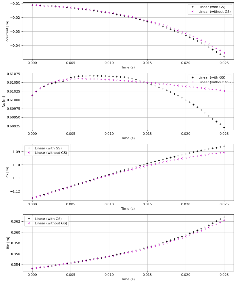
Now we can compare the difference between the linear evolution with and without GS solves at each step. We see that for some parameters the evolution diverges very quickly with solving GS!
fig, ax = plt.subplots(4,1, figsize=(10, 12), dpi=80)
ax = ax.flatten()

labels = ["Zcurrent [m]", "Rx [m]", "Zx [m]", "Rin [m]"]

for i in range(4):
    ax[i].plot(history_times_with_GS, history_plasma_descriptors_with_GS[:, i], 'k+', label="Linear (with GS)")
    ax[i].plot(history_times, history_plasma_descriptors[:, i], 'm3', label="Linear (without GS)")
    ax[i].set_xlabel("Time (s)")
    ax[i].set_ylabel(labels[i])
    ax[i].legend()
    ax[i].grid()

fig.tight_layout()