Example: Extracting a state-space model from an equilibrium
This notebook builds a self-contained MAST-U-like equilibrium, then constructs and inspects the FreeGSNKE state-space model. This is useful for magnetic control design.
Build the equilibrium
import matplotlib.pyplot as plt
import numpy as np

# build machine
from freegsnke import build_machine
tokamak = build_machine.tokamak(
    active_coils_path=f"../machine_configs/MAST-U/MAST-U_like_active_coils.pickle",
    passive_coils_path=f"../machine_configs/MAST-U/MAST-U_like_passive_coils.pickle",
    limiter_path=f"../machine_configs/MAST-U/MAST-U_like_limiter.pickle",
    wall_path=f"../machine_configs/MAST-U/MAST-U_like_wall.pickle",
)

# initialise equilibrium object
from freegsnke import equilibrium_update
eq = equilibrium_update.Equilibrium(
    tokamak=tokamak,
    Rmin=0.1, Rmax=2.0,   # radial range
    Zmin=-2.2, Zmax=2.2,  # vertical range
    nx=65,                # number of grid points in the radial direction (needs to be of the form (2**n + 1) with n being an integer)
    ny=129,               # number of grid points in the vertical direction (needs to be of the form (2**n + 1) with n being an integer)
    # psi=plasma_psi
)

# initialise profile object
from freegsnke.jtor_update import ConstrainPaxisIp
profiles = ConstrainPaxisIp(
    eq=eq,
    paxis=8.1e3,
    Ip=6.2e5,
    fvac=0.5,
    alpha_m=1.8,
    alpha_n=1.2
)

# initialise solver
from freegsnke import GSstaticsolver
GSStaticSolver = GSstaticsolver.NKGSsolver(eq)

# set coil currents
import pickle
with open('data/simple_diverted_currents_PaxisIp.pk', 'rb') as f:
    current_values = pickle.load(f)

for key in current_values.keys():
    eq.tokamak[key].current = current_values[key]
eq.tokamak["P6"].current += 500

# carry out forward solve
GSStaticSolver.solve(eq=eq,
                     profiles=profiles,
                     constrain=None,
                     target_relative_tolerance=1e-9)

# plot the resulting equilibrium
fig1, ax1 = plt.subplots(1, 1, figsize=(4, 8), dpi=80)
ax1.grid(True, which='both')
eq.plot(axis=ax1, show=False)
eq.tokamak.plot(axis=ax1, show=False)
ax1.set_xlim(0.1, 2.15)
ax1.set_ylim(-2.25, 2.25)
plt.tight_layout()
Active coils --> built from pickle file.
Passive structures --> built from pickle file.
Limiter --> built from pickle file.
Wall --> built from pickle file.
Magnetic probes --> none provided.
Resistance (R) and inductance (M) matrices --> built using actives (and passives if present).
Tokamak built.
Forward static solve SUCCESS. Tolerance 4.04e-10 (vs. requested 1.00e-09) reached in 26/100 iterations.
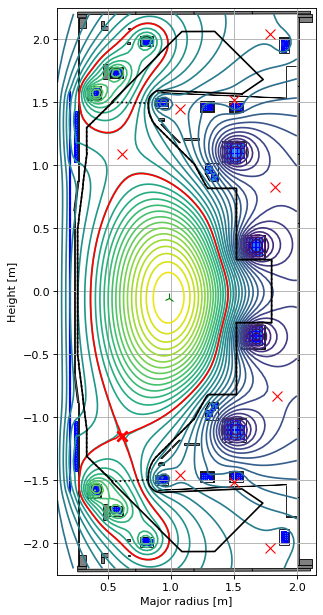
Calculate state space model quantites
Instantiate the nonlinear solver object in order to calculate the state space model matrices and growth rate parameters (and stability margin) for this equilibrium.
Next you need to choose the properties you want for the state-space model. I would encourage you to read the Example10 notebook on the FreeGSNKE repo to see the different settings below. It basically determines how many passive structure modes you wish to use in the model - below I’ve selected to use all the modes (which is a bit slow).
from freegsnke import nonlinear_solve

state_space_model = nonlinear_solve.nl_solver(
    eq=eq,
    profiles=profiles,
    GSStaticSolver=GSStaticSolver,
    plasma_resistivity=2e-7,      # set an appropriate plasma resistivity (goes into the Ip equation)
    # min_dIy_dI=1e-5,            # set between [0,1]
    # threshold_dIy_dI=1,         # set between [0,1]
    # max_mode_frequency=1e10,    # set between [0,inf]
    fix_n_vessel_modes=138,       # retain all passive modes in the MAST-U-like machine
    # custom_coil_resist=coil_R,    # use calibrated resistance matrix for active coils
    # custom_self_ind=coil_M,       # use calibrated inductance matrix for active coils
    n_linearization_workers=6,   # set >1 to parallelise Jacobian construction (i.e. number of cores to use)
    )
-----
Checking that the provided 'eq' and 'profiles' are a GS solution...
Forward static solve SUCCESS. Tolerance 4.04e-10 (vs. requested 1.00e-08) reached in 0/100 iterations.
-----
Instantiating nonlinear solver objects...
done.
-----
Identifying mode selection criteria...
      'fix_n_vessel_modes' option selected --> passive structure modes that couple most to the strongest passive structure mode are being selected.
-----
Initial mode selection:
   Active coils
      total selected = 12 (out of 12)
   Passive structures
      138 selected using 'fix_n_vessel_modes'
   Total number of modes = 150 (12 active coils + 138 passive structures)
      (Note: some additional modes may be removed after Jacobian calculation if 'mode_removal=True')
-----
Building the 3051 x 151 Jacobian (dIy/dI) of plasma current density (inside the LCFS) with respect to all metal currents and the total plasma current.
Building the 3051 x 3 Jacobian (dIy/dtheta) of plasma current density (inside the LCFS) with respect to all plasma current density profile parameters within Jtor.
Built the 1 x 151 Jacobian (ds/dI) of plasma descriptors with respect to all metal currents and the total plasma current.
Built the 1 x 3 Jacobian (ds/dtheta) of plasma descriptors with respect to all plasma current density profile parameters within Jtor.
-----
Stability paramters:
   Deformable plasma metrics:
      Growth rate = [46.0510693] [1/s]
      Instability timescale = [0.02171502] [s]
      Inductive stability margin = [0.7855679+0.j]
   Rigid plasma metrics:
      Leuer parameter (ratio of stabilsing to de-stabilising force gradients):
          between all metals and all metals = 1.87005932947542
          between all metals and active metals = 1.87005932947542
          between passive metals and active metals = 1.8700417105480602
-----
Evolutive solver timestep:
      Solver timestep 'dt_step' has been set to 0.0001 as requested.
      Ensure it is smaller than the growth rate else you may find numerical instability in any subsequent evoltuive simulations!
-----
print(f"Deformable GR = {state_space_model.linearised_sol.growth_rates}")
print(f"Deformable GR (without Ip) = {state_space_model.linearised_sol.growth_rates_const_Ip}")
print(f"Inductive stability margin = {state_space_model.linearised_sol.stability_margin}")
print(f"Leuer parameter = {state_space_model.Leuer_metals_stab_over_active_destab}")
Deformable GR = [46.0510693]
Deformable GR (without Ip) = [42.27904617]
Inductive stability margin = [0.7855679+0.j]
Leuer parameter = 1.87005932947542
Now let’s extract the matrices used in the FreeGSNKE state space model. Below is a (lengthy) recap of the equations that we use:
Assume we have solved the Grad-Shafranov equation and have obtained an equilibrium. From this we can extract the plasma current density discretised over the spatial domain (whose points are only non-zero inside the LCFS, so we mask points outside the limiter to save memory):
This is a function of the:
currents in the metal conductors \(\vec{I}_m\) (i.e. the active coils and passive - or passive modes if we’ve done the decomposition).
plasma current \(I_p\).
parameters \(\vec{\theta}\) used to define the plasma current density profiles (i.e. \(p'(\psi_n)\) and \(FF'(\psi_n)\)).
In order to estimate the instability timescales/growth rates of this plasma, we will need to define (and then linearise) the coupled circuit and plasma equations.
Circuit equations:
These equations govern the flow of current in the active coils and passive structures (while being coupled to the currents in the plasma):
\(M_{m,m}\) is the symmetric matrix of mutual inductances between all of the metals.
\(M_{m,y}\) is the matrix of mutual inductances between all of the metals and the discretised plasma current density.
\(R_{m,m}\) is the diagonal matrix of resistances in the metals.
\(V_m\) is the vector of voltages applied to the metals (note: these are non-zero for the active coils only).
Note that the dots indicate time derivatives.
Plasma equation:
This equation governs the flow of current in the plasma (while being coupled to the currents in the metals):
\(M_{y,m} = M_{m,y}^{T}\) (from above).
\(R_{y,y} = 2 \pi \sigma_p \hat{R} /dA\) is the diagonal matrix of resistances for each plasma element.
\(\sigma_p\) is the assigned plasma resistivity.
\(\hat{R}\) is a matrix storing the radial position of each plasma element.
\(dA\) is the area of each plasma element.
Linearisation of discretised plasma current density:
To simplify these equations, we linearise equation (1) around the current GS equilibrium such that:
The partial derivative terms (i.e. the Jacobians) are calculated in FreeGSNKE using finite differences. The use of these Jacobians is what makes this a deformable growth rate model.
We can plug this equation into both (2) and (3) and re-arrange:
Next, we need to write this in state matrix form. For this, we need to remove the dependence of equation (6) on the denominator \(I_p\) by introducing two terms:
\(\hat{\vec{I}}_y = \vec{I}_y / I_p\) is the normalised discretised plasma current density over the spatial domain.
\(R_p = \hat{\vec{I}}_y^{T} R_{y,y} \hat{\vec{I}}_y\) is the “lumped” plasma resistance.
This results in the state matrix system \(\vec{M} \dot{\vec{x}} + \vec{R} \vec{x} = \vec{c}\):
Note that in the next section we use \(\vec{I}_d\) to represent the vector of active coil and passive mode currents such that \(\vec{I}_m = P \vec{I}_d\) (where \(P\) is the eigenmode decomposition matrix - see original freegsnke paper for details or Example10 notebook).
Also note that you can ignore the effect of the final term on the right hand side of the equation (involving Jacobians wrt the plasma parameters) if so desired - these effects are thought to be small.
State space model:
This can be written as:
where:
\(\vec{x}\) is the state space vector.
\(L_*\) is the modified inductance matrix.
\(R\) is the resistance matrix.
\(u\) is the control (voltage) vector.
Let’s look at the state space vector, which is made up of the:
12 active coil currents [A].
138 passive structure currents [A] (assuming all modes being used).
plasma current [kA] (single number).
The exact ordering is available from the machine object below.
# state space vector
x = state_space_model.currents_vec
print(x.shape)

# ordering of the actives, passives, and Ip in the vector
ordering = tokamak.coil_names
ordering
(151,)
['Solenoid',
 'PX',
 'D1',
 'D2',
 'D3',
 'Dp',
 'D5',
 'D6',
 'D7',
 'P4',
 'P5',
 'P6',
 'vessel_1',
 'vessel_2',
 'vessel_3',
 'vessel_4',
 'vessel_5',
 'vessel_6',
 'vessel_7',
 'vessel_8',
 'vessel_9',
 'vessel_10',
 'vessel_11',
 'vessel_12',
 'vessel_13',
 'vessel_14',
 'vessel_15',
 'vessel_16',
 'vessel_17',
 'vessel_18',
 'vessel_19',
 'vessel_20',
 'vessel_21',
 'vessel_22',
 'centrecolumn_1',
 'centrecolumn_2',
 'centrecolumn_3',
 'centrecolumn_4',
 'centrecolumn_5',
 'centrecolumn_6',
 'centrecolumn_7',
 'centrecolumn_8',
 'centrecolumn_9',
 'centrecolumn_10',
 'colosseum_upper_1',
 'colosseum_upper_2',
 'colosseum_upper_3',
 'colosseum_lower_1',
 'colosseum_lower_2',
 'colosseum_lower_3',
 'colosseum_outer_upper_1',
 'colosseum_outer_upper_2',
 'colosseum_outer_lower_1',
 'colosseum_outer_lower_2',
 'ring_plate_minor_upper_1',
 'ring_plate_minor_upper_2',
 'ring_plate_minor_lower_1',
 'ring_plate_minor_lower_2',
 'ring_plate_major_upper_1',
 'ring_plate_major_lower_1',
 'psp_upper_1',
 'psp_lower_1',
 'gas_baffle_upper_1',
 'gas_baffle_upper_2',
 'gas_baffle_upper_3',
 'gas_baffle_lower_1',
 'gas_baffle_lower_2',
 'gas_baffle_lower_3',
 'd1_case_upper_0',
 'd1_case_upper_1',
 'd1_case_upper_2',
 'd1_case_upper_3',
 'd1_case_lower_0',
 'd1_case_lower_1',
 'd1_case_lower_2',
 'd1_case_lower_3',
 'd2_case_upper_0',
 'd2_case_upper_1',
 'd2_case_upper_2',
 'd2_case_upper_3',
 'd2_case_lower_0',
 'd2_case_lower_1',
 'd2_case_lower_2',
 'd2_case_lower_3',
 'd3_case_upper_0',
 'd3_case_upper_1',
 'd3_case_upper_2',
 'd3_case_upper_3',
 'd3_case_lower_0',
 'd3_case_lower_1',
 'd3_case_lower_2',
 'd3_case_lower_3',
 'd5_case_upper_0',
 'd5_case_upper_1',
 'd5_case_upper_2',
 'd5_case_upper_3',
 'd5_case_lower_0',
 'd5_case_lower_1',
 'd5_case_lower_2',
 'd5_case_lower_3',
 'd6_case_upper_0',
 'd6_case_upper_1',
 'd6_case_upper_2',
 'd6_case_upper_3',
 'd6_case_lower_0',
 'd6_case_lower_1',
 'd6_case_lower_2',
 'd6_case_lower_3',
 'd7_case_upper_0',
 'd7_case_upper_1',
 'd7_case_upper_2',
 'd7_case_upper_3',
 'd7_case_lower_0',
 'd7_case_lower_1',
 'd7_case_lower_2',
 'd7_case_lower_3',
 'dp_case_upper_0',
 'dp_case_upper_1',
 'dp_case_upper_2',
 'dp_case_upper_3',
 'dp_case_lower_0',
 'dp_case_lower_1',
 'dp_case_lower_2',
 'dp_case_lower_3',
 'p4_case_upper_0',
 'p4_case_upper_1',
 'p4_case_upper_2',
 'p4_case_upper_3',
 'p4_case_lower_0',
 'p4_case_lower_1',
 'p4_case_lower_2',
 'p4_case_lower_3',
 'p5_case_upper_0',
 'p5_case_upper_1',
 'p5_case_upper_2',
 'p5_case_upper_3',
 'p5_case_lower_0',
 'p5_case_lower_1',
 'p5_case_lower_2',
 'p5_case_lower_3',
 'p6_case_upper_0',
 'p6_case_upper_1',
 'p6_case_upper_2',
 'p6_case_upper_3',
 'p6_case_upper_4',
 'p6_case_lower_0',
 'p6_case_lower_1',
 'p6_case_lower_2',
 'p6_case_lower_3',
 'p6_case_lower_4']
# mutual inductances between all metals
Mmm = state_space_model.evol_metal_curr.coil_self_ind
print(Mmm.shape)

# resistances for all metals
Rmm = state_space_model.evol_metal_curr.coil_resist
print(Rmm.shape)

# mutual inductances between all metals and plasma grid elements
Mmy = state_space_model.evol_metal_curr.Mey_matrix
print(Mmy.shape)

# normalised plasma current density (Iy / Ip), sums to 1, defined over the same plasma-grid elements as Iy
hatIy = state_space_model.hatIy
print(hatIy.shape)

# Myy @ hatIy, precomputed by FreeGSNKE without ever forming the full Myy matrix
# (Myy itself is only ever built/stored on a small adaptive sub-domain around the plasma - see state_space_model.handleMyy)
Myy_hatIy = state_space_model.Myy_hatIy0
print(Myy_hatIy.shape)
(150, 150)
(150,)
(150, 3051)
(3051,)
(3051,)
# mode transformation matrix (if number of passive modes reduced)
P = state_space_model.linearised_sol.P
P.shape
(150, 150)
# Jacobian of plasma current density wrt mode currents (i.e. the linearisation!)
dIydId = state_space_model.linearised_sol.dIydI[:,0:-1]
print(dIydId.shape)

# Jacobian of plasma current density wrt plasma current (i.e. the linearisation!)
dIydIp = state_space_model.linearised_sol.dIydI[:,-1] / state_space_model.plasma_norm_factor
print(dIydIp.shape)
(3051, 150)
(3051,)
# diagonal of R_yy, the plasma resistance matrix (2*pi*sigma_p*Rhat/dA), one entry per plasma grid point
Ryy = state_space_model.plasma_resistance_1d
print(Ryy.shape)

# lumped plasma resistance: Rp = hatIy^T @ Ryy @ hatIy
Rp = np.dot(Ryy, hatIy**2)
print(Rp)
(3051,)
9.439922892246269e-07
Assemble \(L_*\) and \(R\)
Substituting \(\vec{I}_m = P \vec{I}_d\) into the block matrix above (so that the state vector becomes \(\vec{x} = (\vec{I}_d, I_p)^T\), matching state_space_model.currents_vec) gives:
where \(A = \partial \vec{I}_y/\partial \vec{I}_d\) (dIydId) and \(B = \partial \vec{I}_y/\partial I_p\) (dIydIp).
Two things to watch for when using the quantities already extracted above:
\(\hat{\vec I}_y^{T} M_{y,y} = (M_{y,y}\hat{\vec I}_y)^{T}\) since \(M_{y,y}\) is symmetric, so both bottom-row terms can be built from the vector
Myy_hatIy0alone (Myy_hatIy0 @ AandMyy_hatIy0 @ B) - we never need the full \(M_{y,y}\) matrix.
n = P.shape[0]   # number of independent active-coil and passive-structure modes

# L* blocks
L_dd = Mmm @ P + Mmy @ dIydId                       # (n, n)
L_dp = Mmy @ dIydIp                                 # (n,)
L_pd = (Myy_hatIy @ dIydId + (Mmy @ hatIy) @ P) / Rp   # (n,)
L_pp = (Myy_hatIy @ dIydIp) / Rp                   # scalar

L_star = np.zeros((n + 1, n + 1))
L_star[:n, :n] = L_dd
L_star[:n, -1] = L_dp
L_star[-1, :n] = L_pd
L_star[-1, -1] = L_pp

# R blocks
R = np.zeros((n + 1, n + 1))
R[:n, :n] = np.diag(Rmm) @ P
R[-1, -1] = 1.0

L_star.shape, R.shape
((151, 151), (151, 151))
Sanity check against FreeGSNKE’s own growth rates
\(L_* \dot{\vec x} + R \vec x = \vec u\) implies \(\dot{\vec x} = -L_*^{-1}R\,\vec x + L_*^{-1}\vec u\), so the eigenvalues of \(-L_*^{-1}R\) are the system’s characteristic (growth) rates.
This should match state_space_model.linearised_sol.growth_rates (up to which of the eigenvalues are unstable/positive), independently of the internal basis/scaling FreeGSNKE itself uses to build linearised_sol.Mmatrix.
Note that FreeGSNKE internally calculates the GRs using \(-R^{-1} L_*\) as it’s more numerically stable so we’ll do that here.
# P inverse
Pm1 = state_space_model.evol_metal_curr.Pm1

# find R^{-1} @ L*
Rinv_L = np.zeros_like(L_star)
Rinv_L[:n, :] = (Pm1 @ np.diag(1.0 / Rmm)) @ L_star[:n, :]   # R_dd^-1 @ [L_dd | L_dp]
Rinv_L[-1, :] = L_star[-1, :]                                # R_pp = 1, so this row is unchanged

# eigenvalues of R^-1 L* are reciprocals of eigenvalues of L*^-1 R, so growth_rate = -1/eigenvalue
timescales = -np.linalg.eigvals(Rinv_L)
growth_rates = np.sort(1.0 / timescales[timescales.real > 0].real)

print("Growth rates from L_*, R assembled here:", growth_rates)
print("Growth rates from state_space_model:    ", state_space_model.linearised_sol.growth_rates.real)
Growth rates from L_*, R assembled here: [46.0510693]
Growth rates from state_space_model:     [46.0510693]